Strongly regular graph

Last updated
The Paley graph of order 13, a strongly regular graph with parameters srg(13,6,2,3). Paley13.svg
The Paley graph of order 13, a strongly regular graph with parameters srg(13,6,2,3).
Graph families defined by their automorphisms
distance-transitive distance-regular strongly regular
symmetric (arc-transitive) t-transitive,t  2 skew-symmetric
(if connected)
vertex- and edge-transitive
edge-transitive and regular edge-transitive
vertex-transitive regular (if bipartite)
biregular
Cayley graph zero-symmetric asymmetric

In graph theory, a strongly regular graph (SRG) is a regular graph G = (V, E) with v vertices and degree k such that

Contents

for some integers

The complement of a strongly regular graph is also strongly regular. The complement of an srg(v, k, λ, μ) is an srg(v, vk − 1, v − 2 − 2k + μ, v − 2k + λ).

A strongly regular graph is a distance-regular graph with diameter 2 whenever μ is non-zero. It is a locally linear graph whenever λ = 1.

Etymology

A strongly regular graph is denoted an srg(v, k, λ, μ) in the literature. By convention, graphs which satisfy the definition trivially are excluded from detailed studies and lists of strongly regular graphs. These include the disjoint union of one or more equal-sized complete graphs, [1] [2] and their complements, the complete multipartite graphs with equal-sized independent sets.

Andries Brouwer and Hendrik van Maldeghem (see #References) use an alternate but fully equivalent definition of a strongly regular graph based on spectral graph theory: a strongly regular graph is a finite regular graph that has exactly three eigenvalues, only one of which is equal to the degree k, of multiplicity 1. This automatically rules out fully connected graphs (which have only two distinct eigenvalues, not three) and disconnected graphs (whose multiplicity of the degree k is equal to the number of different connected components, which would therefore exceed one). Much of the literature, including Brouwer, refer to the larger eigenvalue as r (with multiplicity f) and the smaller one as s (with multiplicity g).

History

Strongly regular graphs were introduced by R.C. Bose in 1963. [3] They built upon earlier work in the 1950s in the then-new field of spectral graph theory.

Examples

A strongly regular graph is called primitive if both the graph and its complement are connected. All the above graphs are primitive, as otherwise μ = 0 or λ = k.

Conway's 99-graph problem asks for the construction of an srg(99, 14, 1, 2). It is unknown whether a graph with these parameters exists, and John Horton Conway offered a $1000 prize for the solution to this problem. [5]

Triangle-free graphs

The strongly regular graphs with λ = 0 are triangle free. Apart from the complete graphs on fewer than 3 vertices and all complete bipartite graphs, the seven listed earlier (pentagon, Petersen, Clebsch, Hoffman-Singleton, Gewirtz, Mesner-M22, and Higman-Sims) are the only known ones.

Geodetic graphs

Every strongly regular graph with is a geodetic graph, a graph in which every two vertices have a unique unweighted shortest path. [6] The only known strongly regular graphs with are those where is 0, therefore triangle-free as well. These are called the Moore graphs and are explored below in more detail. Other combinations of parameters such as (400, 21, 2, 1) have not yet been ruled out. Despite ongoing research on the properties that a strongly regular graph with would have, [7] [8] it is not known whether any more exist or even whether their number is finite. [6] Only the elementary result is known, that cannot be 1 for such a graph.

Algebraic properties of strongly regular graphs

Basic relationship between parameters

The four parameters in an srg(v, k, λ, μ) are not independent. They must obey the following relation:

The above relation is derived through a counting argument as follows:

  1. Imagine the vertices of the graph to lie in three levels. Pick any vertex as the root, in Level 0. Then its k neighbors lie in Level 1, and all other vertices lie in Level 2.
  2. Vertices in Level 1 are directly connected to the root, hence they must have λ other neighbors in common with the root, and these common neighbors must also be in Level 1. Since each vertex has degree k, there are edges remaining for each Level 1 node to connect to vertices in Level 2. Therefore, there are edges between Level 1 and Level 2.
  3. Vertices in Level 2 are not directly connected to the root, hence they must have μ common neighbors with the root, and these common neighbors must all be in Level 1. There are vertices in Level 2, and each is connected to μ vertices in Level 1. Therefore the number of edges between Level 1 and Level 2 is .
  4. Equating the two expressions for the edges between Level 1 and Level 2, the relation follows.

Adjacency matrix equations

Let I denote the identity matrix and let J denote the matrix of ones, both matrices of order v. The adjacency matrix A of a strongly regular graph satisfies two equations.

First:

which is a restatement of the regularity requirement. This shows that k is an eigenvalue of the adjacency matrix with the all-ones eigenvector.

Second:

which expresses strong regularity. The ij-th element of the left hand side gives the number of two-step paths from i to j. The first term of the right hand side gives the number of two-step paths from i back to i, namely k edges out and back in. The second term gives the number of two-step paths when i and j are directly connected. The third term gives the corresponding value when i and j are not connected. Since the three cases are mutually exclusive and collectively exhaustive, the simple additive equality follows.

Conversely, a graph whose adjacency matrix satisfies both of the above conditions and which is not a complete or null graph is a strongly regular graph. [9]

Eigenvalues and graph spectrum

Since the adjacency matrix A is symmetric, it follows that its eigenvectors are orthogonal. We already observed one eigenvector above which is made of all ones, corresponding to the eigenvalue k. Therefore the other eigenvectors x must all satisfy where J is the all-ones matrix as before. Take the previously established equation:

and multiply the above equation by eigenvector x:

Call the corresponding eigenvalue p (not to be confused with the graph parameter) and substitute , and :

Eliminate x and rearrange to get a quadratic:

This gives the two additional eigenvalues . There are thus exactly three eigenvalues for a strongly regular matrix.

Conversely, a connected regular graph with only three eigenvalues is strongly regular. [10]

Following the terminology in much of the strongly regular graph literature, the larger eigenvalue is called r with multiplicity f and the smaller one is called s with multiplicity g.

Since the sum of all the eigenvalues is the trace of the adjacency matrix, which is zero in this case, the respective multiplicities f and g can be calculated:

As the multiplicities must be integers, their expressions provide further constraints on the values of v, k, μ, and λ.

Strongly regular graphs for which have integer eigenvalues with unequal multiplicities.

Strongly regular graphs for which are called conference graphs because of their connection with symmetric conference matrices. Their parameters reduce to

Their eigenvalues are and , both of whose multiplicities are equal to . Further, in this case, v must equal the sum of two squares, related to the Bruck–Ryser–Chowla theorem.

Further properties of the eigenvalues and their multiplicities are:

If the above condition(s) are violated for any set of parameters, then there exists no strongly regular graph for those parameters. Brouwer has compiled such lists of existence or non-existence here with reasons for non-existence if any.

The Hoffman–Singleton theorem

As noted above, the multiplicities of the eigenvalues are given by

which must be integers.

In 1960, Alan Hoffman and Robert Singleton examined those expressions when applied on Moore graphs that have λ = 0 and μ = 1. Such graphs are free of triangles (otherwise λ would exceed zero) and quadrilaterals (otherwise μ would exceed 1), hence they have a girth (smallest cycle length) of 5. Substituting the values of λ and μ in the equation , it can be seen that , and the eigenvalue multiplicities reduce to

For the multiplicities to be integers, the quantity must be rational, therefore either the numerator is zero or the denominator is an integer.

If the numerator is zero, the possibilities are:

If the denominator is an integer t, then is a perfect square , so . Substituting:

Since both sides are integers, must be an integer, therefore t is a factor of 15, namely , therefore . In turn:

The Hoffman-Singleton theorem states that there are no strongly regular girth-5 Moore graphs except the ones listed above.

See also

Notes

  1. Brouwer, Andries E; Haemers, Willem H. Spectra of Graphs. p. 101 Archived 2012-03-16 at the Wayback Machine
  2. Godsil, Chris; Royle, Gordon. Algebraic Graph Theory. Springer-Verlag New York, 2001, p. 218.
  3. https://projecteuclid.org/euclid.pjm/1103035734, R. C. Bose, Strongly regular graphs, partial geometries and partially balanced designs, Pacific J. Math 13 (1963) 389–419. (p. 122)
  4. Weisstein, Eric W., "Schläfli graph", MathWorld
  5. Conway, John H., Five $1,000 Problems (Update 2017) (PDF), Online Encyclopedia of Integer Sequences, retrieved 2019-02-12
  6. 1 2 Blokhuis, A.; Brouwer, A. E. (1988), "Geodetic graphs of diameter two", Geometriae Dedicata , 25 (1–3): 527–533, doi:10.1007/BF00191941, MR   0925851, S2CID   189890651
  7. Deutsch, J.; Fisher, P. H. (2001), "On strongly regular graphs with ", European Journal of Combinatorics , 22 (3): 303–306, doi: 10.1006/eujc.2000.0472 , MR   1822718
  8. Belousov, I. N.; Makhnev, A. A. (2006), "On strongly regular graphs with and their automorphisms", Doklady Akademii Nauk , 410 (2): 151–155, MR   2455371
  9. Cameron, P.J.; van Lint, J.H. (1991), Designs, Graphs, Codes and their Links, London Mathematical Society Student Texts 22, Cambridge University Press, p.  37, ISBN   978-0-521-42385-4
  10. Godsil, Chris; Royle, Gordon. Algebraic Graph Theory. Springer-Verlag, New York, 2001, Lemma 10.2.1.
  11. Dalfó, C. (2019), "A survey on the missing Moore graph", Linear Algebra and Its Applications, 569: 1–14, doi:10.1016/j.laa.2018.12.035, hdl: 2117/127212 , MR   3901732, S2CID   126689579

Related Research Articles

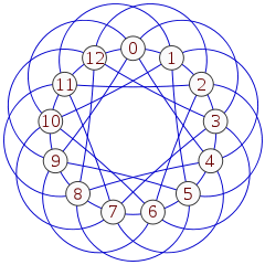
In graph theory, an expander graph is a sparse graph that has strong connectivity properties, quantified using vertex, edge or spectral expansion. Expander constructions have spawned research in pure and applied mathematics, with several applications to complexity theory, design of robust computer networks, and the theory of error-correcting codes.

<span class="mw-page-title-main">Regular graph</span> Graph where each vertex has the same number of neighbors

In graph theory, a regular graph is a graph where each vertex has the same number of neighbors; i.e. every vertex has the same degree or valency. A regular directed graph must also satisfy the stronger condition that the indegree and outdegree of each internal vertex are equal to each other. A regular graph with vertices of degree k is called a k‑regular graph or regular graph of degree k. Also, from the handshaking lemma, a regular graph contains an even number of vertices with odd degree.

<span class="mw-page-title-main">Legendre function</span>

In physical science and mathematics, the Legendre functionsPλ, Qλ and associated Legendre functionsPμ
λ
, Qμ
λ
, and Legendre functions of the second kind, Qn, are all solutions of Legendre's differential equation. The Legendre polynomials and the associated Legendre polynomials are also solutions of the differential equation in special cases, which, by virtue of being polynomials, have a large number of additional properties, mathematical structure, and applications. For these polynomial solutions, see the separate Wikipedia articles.

In graph theory and computer science, an adjacency matrix is a square matrix used to represent a finite graph. The elements of the matrix indicate whether pairs of vertices are adjacent or not in the graph.

In mathematics, spectral graph theory is the study of the properties of a graph in relationship to the characteristic polynomial, eigenvalues, and eigenvectors of matrices associated with the graph, such as its adjacency matrix or Laplacian matrix.

In quantum field theory, a quartic interaction is a type of self-interaction in a scalar field. Other types of quartic interactions may be found under the topic of four-fermion interactions. A classical free scalar field satisfies the Klein–Gordon equation. If a scalar field is denoted , a quartic interaction is represented by adding a potential energy term to the Lagrangian density. The coupling constant is dimensionless in 4-dimensional spacetime.

In mathematics, the discrete Laplace operator is an analog of the continuous Laplace operator, defined so that it has meaning on a graph or a discrete grid. For the case of a finite-dimensional graph, the discrete Laplace operator is more commonly called the Laplacian matrix.

<span class="mw-page-title-main">Bethe lattice</span>

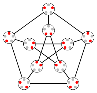
In statistical mechanics and mathematics, the Bethe lattice is an infinite connected cycle-free graph where all vertices have the same number of neighbors. The Bethe lattice was introduced into the physics literature by Hans Bethe in 1935. In such a graph, each node is connected to z neighbors; the number z is called either the coordination number or the degree, depending on the field.

In linear algebra, an eigenvector or characteristic vector of a linear transformation is a nonzero vector that changes at most by a constant factor when that linear transformation is applied to it. The corresponding eigenvalue, often represented by , is the multiplying factor.

<span class="mw-page-title-main">Noncentral chi-squared distribution</span>

In probability theory and statistics, the noncentral chi-squared distribution is a noncentral generalization of the chi-squared distribution. It often arises in the power analysis of statistical tests in which the null distribution is a chi-squared distribution; important examples of such tests are the likelihood-ratio tests.

<span class="mw-page-title-main">Generalized inverse Gaussian distribution</span>

In probability theory and statistics, the generalized inverse Gaussian distribution (GIG) is a three-parameter family of continuous probability distributions with probability density function

<span class="mw-page-title-main">Kneser graph</span> Graph whose vertices correspond to combinations of a set of n elements

In graph theory, the Kneser graphK(n, k) (alternatively KGn,k) is the graph whose vertices correspond to the k-element subsets of a set of n elements, and where two vertices are adjacent if and only if the two corresponding sets are disjoint. Kneser graphs are named after Martin Kneser, who first investigated them in 1956.

<span class="mw-page-title-main">Inverse Gaussian distribution</span> Family of continuous probability distributions

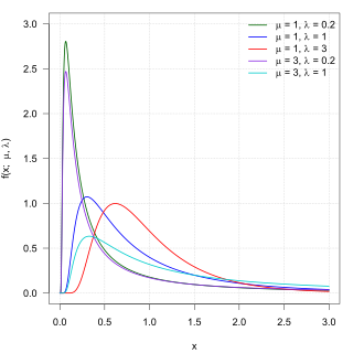
In probability theory, the inverse Gaussian distribution is a two-parameter family of continuous probability distributions with support on (0,∞).

In graph theory, a graph is said to be a pseudorandom graph if it obeys certain properties that random graphs obey with high probability. There is no concrete definition of graph pseudorandomness, but there are many reasonable characterizations of pseudorandomness one can consider.

The expander mixing lemma intuitively states that the edges of certain -regular graphs are evenly distributed throughout the graph. In particular, the number of edges between two vertex subsets and is always close to the expected number of edges between them in a random -regular graph, namely .

In the mathematical discipline of graph theory, the expander walk sampling theorem intuitively states that sampling vertices in an expander graph by doing relatively short random walk can simulate sampling the vertices independently from a uniform distribution. The earliest version of this theorem is due to Ajtai, Komlós & Szemerédi (1987), and the more general version is typically attributed to Gillman (1998).

In physics and mathematics, the solid harmonics are solutions of the Laplace equation in spherical polar coordinates, assumed to be (smooth) functions . There are two kinds: the regular solid harmonics, which are well-defined at the origin and the irregular solid harmonics, which are singular at the origin. Both sets of functions play an important role in potential theory, and are obtained by rescaling spherical harmonics appropriately:

In mathematics, the spectral theory of ordinary differential equations is the part of spectral theory concerned with the determination of the spectrum and eigenfunction expansion associated with a linear ordinary differential equation. In his dissertation, Hermann Weyl generalized the classical Sturm–Liouville theory on a finite closed interval to second order differential operators with singularities at the endpoints of the interval, possibly semi-infinite or infinite. Unlike the classical case, the spectrum may no longer consist of just a countable set of eigenvalues, but may also contain a continuous part. In this case the eigenfunction expansion involves an integral over the continuous part with respect to a spectral measure, given by the Titchmarsh–Kodaira formula. The theory was put in its final simplified form for singular differential equations of even degree by Kodaira and others, using von Neumann's spectral theorem. It has had important applications in quantum mechanics, operator theory and harmonic analysis on semisimple Lie groups.

<span class="mw-page-title-main">Marchenko–Pastur distribution</span> Distribution of singular values of large rectangular random matrices

In the mathematical theory of random matrices, the Marchenko–Pastur distribution, or Marchenko–Pastur law, describes the asymptotic behavior of singular values of large rectangular random matrices. The theorem is named after Soviet mathematicians Vladimir Marchenko and Leonid Pastur who proved this result in 1967.

In spectral graph theory, the Alon–Boppana bound provides a lower bound on the second-largest eigenvalue of the adjacency matrix of a -regular graph, meaning a graph in which every vertex has degree . The reason for the interest in the second-largest eigenvalue is that the largest eigenvalue is guaranteed to be due to -regularity, with the all-ones vector being the associated eigenvector. The graphs that come close to meeting this bound are Ramanujan graphs, which are examples of the best possible expander graphs.

References