Directivity

Diagram showing directivity: the highest power density of this antenna is in the direction of the red lobe

In electromagnetics, directivity is a parameter of an antenna or optical system which measures the degree to which the radiation emitted is concentrated in a single direction. It is the ratio of the radiation intensity in a given direction from the antenna to the radiation intensity averaged over all directions. ^[1] Therefore, the directivity of a hypothetical isotropic radiator is 1, or 0 dBi.

An antenna's directivity is greater than its gain by an efficiency factor, radiation efficiency. ^[1] Directivity is an important measure because many antennas and optical systems are designed to radiate electromagnetic waves in a single direction or over a narrow-angle. By the principle of reciprocity, the directivity of an antenna when receiving is equal to its directivity when transmitting.

The directivity of an actual antenna can vary from 1.76 dBi for a short dipole to as much as 50 dBi for a large dish antenna. ^[2]

Definition

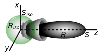
Diagram illustrating how directivity is defined. It shows the radiation pattern of a directional antenna (R, grey) that radiates maximum power along the z-axis, and the pattern of an isotropic antenna (R_iso, green) with the same total radiated power. The directivity is defined as the ratio of the maximum signal strength S radiated by the antenna to the signal strength S_iso radiated by the isotropic antenna

$${\displaystyle G={S \over S_{\text{iso}}}}$$

Since the directional antenna radiates most of its power into a small solid angle around the z-axis its maximum signal strength is much larger than the isotropic antenna which spreads the same power in all directions. Thus the directivity ${\displaystyle G}$ is much greater than one.

The directivity, ${\displaystyle D}$, of an antenna is defined for all incident angles of an antenna. The term "directive gain" is deprecated by IEEE. If an angle relative to the antenna is not specified, then directivity is presumed to refer to the axis of maximum radiation intensity. ^[1]

${\displaystyle D(\theta ,\phi )={\frac {U(\theta ,\phi )}{P_{\text{tot}}/\left(4\pi \right)}}.}$

Here ${\displaystyle \theta }$ and ${\displaystyle \phi }$ are the zenith angle and azimuth angle respectively in the standard spherical coordinate angles; ${\displaystyle U(\theta ,\phi )}$ is the radiation intensity, which is the power per unit solid angle; and ${\displaystyle P_{\text{tot}}}$is the total radiated power. The quantities ${\displaystyle U(\theta ,\phi )}$ and ${\displaystyle P_{\text{tot}}}$ satisfy the relation

${\displaystyle P_{\text{tot}}=\int _{\phi =0}^{\phi =2\pi }\int _{\theta =0}^{\theta =\pi }U\sin \theta \,d\theta \,d\phi$ ;}

that is, the total radiated power ${\displaystyle P_{\text{tot}}}$ is the power per unit solid angle ${\displaystyle U(\theta ,\phi )}$ integrated over a spherical surface. Since there are 4π steradians on the surface of a sphere, the quantity ${\displaystyle P_{\text{tot}}/(4\pi )}$ represents the average power per unit solid angle.

In other words, directivity is the radiation intensity of an antenna at a particular ${\displaystyle (\theta ,\phi )}$ coordinate combination divided by what the radiation intensity would have been had the antenna been an isotropic antenna radiating the same amount of total power into space.

Directivity, if a direction is not specified, is the maximal directive gain value found among all possible solid angles:

${\displaystyle {\begin{aligned}D&=\max \left({\frac {U}{P_{\text{tot}}/\left(4\pi \right)}}\right)\\[3pt]&={\frac {\left.U(\theta ,\phi )\right|_{\text{max}}}{{\frac {1}{4\pi }}\int _{0}^{2\pi }\int _{0}^{\pi }U(\theta ,\phi )\sin \theta \,d\theta \,d\phi }}.\end{aligned}}}$

In antenna arrays

In an antenna array the directivity is a complicated calculation in the general case. For a linear array the directivity will always be less than or equal to the number of elements. For a standard linear array (SLA), where the element spacing is ${\textstyle {\frac {\lambda }{2}}}$, the directivity is equal to the inverse of the square of the 2-norm of the array weight vector, under the assumption that the weight vector is normalized such that its sum is unity. ^[3]

${\displaystyle D_{\text{SLA}}={1 \over {\vec {w}}^{\textsf {H}}{\vec {w}}}\leq N}$

In the case of a uniformly weighted (un-tapered) SLA, this reduces to simply N, the number of array elements.

For a planar array, the computation of directivity is more complicated and requires consideration of the positions of each array element with respect to all the others and with respect to wavelength. ^[4] For a planar rectangular or hexagonally spaced array with non-isotropic elements, the maximum directivity can be estimated using the universal ratio of effective aperture to directivity, ${\textstyle {\frac {\lambda ^{2}}{4\pi }}}$,

${\displaystyle D=A_{e}{4{\pi } \over \lambda ^{2}}=Ndx\,dy\,\eta {4\pi \over \lambda ^{2}}}$

where dx and dy are the element spacings in the x and y dimensions and ${\displaystyle \eta }$ is the "illumination efficiency" of the array that accounts for tapering and spacing of the elements in the array. For an un-tapered array with elements at less than ${\displaystyle \lambda }$ spacing, ${\displaystyle \eta =1}$. Note that for an un-tapered standard rectangular array (SRA), where ${\textstyle dx=dy={\lambda \over 2}}$, this reduces to ${\displaystyle D\approx N\pi }$. For an un-tapered standard rectangular array (SRA), where ${\displaystyle dx=dy=\lambda }$, this reduces to a maximum value of ${\displaystyle D_{\text{max}}\approx 4N\pi }$. The directivity of a planar array is the product of the array gain, and the directivity of an element (assuming all of the elements are identical) only in the limit as element spacing becomes much larger than lambda. In the case of a sparse array, where element spacing ${\displaystyle >\lambda }$, ${\displaystyle \eta }$ is reduced because the array is not uniformly illuminated.

There is a physically intuitive reason for this relationship; essentially there are a limited number of photons per unit area to be captured by the individual antennas. Placing two high gain antennas very close to each other (less than a wavelength) does not buy twice the gain, for example. Conversely, if the antenna are more than a wavelength apart, there are photons that fall between the elements and are not collected at all. This is why the physical aperture size must be taken into account.

Let's assume a 16×16 un-tapered standard rectangular array (which means that elements are spaced at ${\textstyle {\frac {\lambda }{2}}}$.) The array gain is ${\displaystyle 10\log _{10}(N)=10\log _{10}(256)=24.1}$dB. If the array were tapered, this value would go down. The directivity, assuming isotropic elements, is 25.9dBi. ^[5] Now assume elements with 9.0dBi directivity. The directivity is not 33.1dBi, but rather is only 29.2dBi. ^[6] The reason for this is that the effective aperture of the individual elements limits their directivity. So, ${\textstyle D=A_{e}{\frac {4\pi }{\lambda ^{2}}}=Ndx\,dy\,\eta {\frac {4\pi }{\lambda ^{2}}}=N{\frac {\lambda }{2}}{\frac {\lambda }{2}}{\frac {4\pi }{\lambda ^{2}}}=N\pi }$. Note, in this case ${\displaystyle \eta =1}$ because the array is un-tapered. Why the slight difference from ${\displaystyle 10\log _{10}(N\pi )={}}$ 29.05 dBi? The elements around the edge of the array aren't as limited in their effective aperture as are the majority of elements.

Now let's move the array elements to ${\displaystyle \lambda }$ spacing. From the above formula, we expect the directivity to peak at ${\textstyle D=A_{e}{\frac {4\pi }{\lambda ^{2}}}=Ndx\,dy\,\eta {\frac {4\pi }{\lambda ^{2}}}=N\lambda \,\lambda \,{\frac {4\pi }{\lambda ^{2}}}=4N\pi }$. The actual result is 34.6380 dBi, just shy of the ideal 35.0745 dBi we expected. ^[7] Why the difference from the ideal? If the spacing in the x and y dimensions is ${\displaystyle \lambda }$, then the spacing along the diagonals is ${\displaystyle \lambda {\sqrt {2}}}$, thus creating tiny regions in the overall array where photons are missed, leading to ${\displaystyle \eta <1}$.

Now go to ${\displaystyle 10\lambda }$ spacing. The result now should converge to N times the element gain, or ${\displaystyle 10\log _{10}(N)}$ + 9 dBi = 33.1 dBi. The actual result is in fact, 33.1 dBi. ^[8]

For antenna arrays, the closed form expression for Directivity for progressively phased ^[9] array of isotropic sources will be given by, ^[10]

${\displaystyle D={\frac {\left(\sum \limits _{n=1}^{N}I_{n}\right)^{2}}{\sum \limits _{m=1}^{N}\sum \limits _{n=1}^{N}I_{m}I_{n}e^{j(\beta _{m}-\beta _{n})}\operatorname {sinc} {\big (}2r_{mn}{\big )}}}}$

where,

${\displaystyle N}$ is the total number of elements on the aperture;

${\displaystyle \{x_{n},y_{n},z_{n}\}}$ represents the location of elements in Cartesian co-ordinate system;

${\displaystyle I_{n}e^{j\beta _{n}}}$ is the complex excitation coefficient of the ${\displaystyle n^{\textrm {th}}}$-element;

${\displaystyle \beta _{n}=-k(x_{n}\sin \theta _{\tau }\cos \phi _{\tau }+y_{n}\sin \theta _{\tau }\sin \phi _{\tau }+z_{n}\cos \theta _{\tau })}$ is the phase component (progressive phasing);

${\textstyle k={\frac {2\pi }{\lambda }}}$ is the wavenumber;

${\displaystyle \{\theta _{\tau },\phi _{\tau }\}}$ is the angular location of the far-field target;

${\displaystyle r_{mn}={\sqrt {(x_{m}-x_{n})^{2}+(y_{m}-y_{n})^{2}+(z_{m}-z_{n})^{2}}}}$ is the Euclidean distance between the ${\displaystyle m^{\textrm {th}}}$ and ${\displaystyle n^{\textrm {th}}}$ element on the aperture, and

${\textstyle \operatorname {sinc} (x)={\frac {1}{\pi x}}\sin(\pi x)}$

Further studies on directivity expressions for various cases, like if the sources are omnidirectional (even in the array environment) like if the prototype element-pattern takes the form ${\textstyle \sin ^{\mu }\theta \cos ^{\nu }\theta ,\;\left(\mu >-1,\nu >-{\frac {1}{2}}\right)}$, and not restricting to progressive phasing can be done from. ^{[11] [12] [10] [13]}

Relation to beam width

The beam solid angle, represented as ${\displaystyle \Omega _{A}}$, is defined as the solid angle which all power would flow through if the antenna radiation intensity were constant at its maximal value. If the beam solid angle is known, then maximum directivity can be calculated as

${\displaystyle D={\frac {4\pi }{\Omega _{A}}},}$

which simply calculates the ratio of the beam solid angle to the solid angle of a sphere.

The beam solid angle can be approximated for antennas with one narrow major lobe and very negligible minor lobes by simply multiplying the half-power beamwidths (in radians) in two perpendicular planes. The half-power beamwidth is simply the angle in which the radiation intensity is at least half of the peak radiation intensity.

The same calculations can be performed in degrees rather than in radians:

${\displaystyle D\approx 4\pi {\frac {\left({\frac {180}{\pi }}\right)^{2}}{\Theta _{1d}\Theta _{2d}}}\approx {\frac {41253}{\Theta _{1d}\Theta _{2d}}},}$

where ${\displaystyle \Theta _{1d}}$ is the half-power beamwidth in one plane (in degrees) and ${\displaystyle \Theta _{2d}}$ is the half-power beamwidth in a plane at a right angle to the other (in degrees).

In planar arrays, a better approximation is

${\displaystyle D\approx {\frac {32400}{\Theta _{1d}\Theta _{2d}}}.}$

For an antenna with a conical (or approximately conical) beam with a half-power beamwidth of ${\displaystyle \theta }$ degrees, then elementary integral calculus yields an expression for the directivity as

${\displaystyle D={\frac {2}{1-\cos {\frac {\theta }{2}}}}}$.

Expression in decibels

The directivity is rarely expressed as the unitless number ${\displaystyle D}$ but rather as a decibel comparison to a reference antenna:

${\displaystyle D_{\text{dB}}=10\log _{10}\left[{\frac {D}{D_{\text{reference}}}}\right].}$

The reference antenna is usually the theoretical perfect isotropic radiator, which radiates uniformly in all directions and hence has a directivity of 1. The calculation is therefore simplified to

${\displaystyle D_{\text{dBi}}=10\log _{10}D.}$

Another common reference antenna is the theoretical perfect half-wave dipole, which radiates perpendicular to itself with a directivity of 1.64:

${\displaystyle D_{\text{dBd}}\approx 10\log _{10}\left[{\frac {D}{1.64}}\right].}$

Accounting for polarization

When polarization is taken under consideration, three additional measures can be calculated:

Partial directive gain

Partial directive gain is the power density in a particular direction and for a particular component of the polarization, divided by the average power density for all directions and all polarizations. For any pair of orthogonal polarizations (such as left-hand-circular and right-hand-circular), the individual power densities simply add to give the total power density. Thus, if expressed as dimensionless ratios rather than in dB, the total directive gain is equal to the sum of the two partial directive gains. ^[14]

Partial directivity

Partial directivity is calculated in the same manner as the partial directive gain, but without consideration of antenna efficiency (i.e. assuming a lossless antenna). It is similarly additive for orthogonal polarizations.

Partial gain

Main article: Antenna gain

Partial gain is calculated in the same manner as gain, but considering only a certain polarization. It is similarly additive for orthogonal polarizations.

In other areas

The term directivity is also used with other systems.

With directional couplers, directivity is a measure of the difference in dB of the power output at a coupled port, when power is transmitted in the desired direction, to the power output at the same coupled port when the same amount of power is transmitted in the opposite direction. ^[15]

In acoustics, it is used as a measure of the radiation pattern from a source indicating how much of the total energy from the source is radiating in a particular direction. In electro-acoustics, these patterns commonly include omnidirectional, cardioid and hyper-cardioid microphone polar patterns. A loudspeaker with a high degree of directivity (narrow dispersion pattern) can be said to have a high Q. ^[16]

References

1. IEEE Std 145-2013, IEEE Standard for Definitions of Terms for Antennas, IEEE
2. Antenna Tutorial
3. Van Trees, H.L. Optimum Array Processing. pp. 60–63.
4. Van Trees, H.L. Optimum Array Processing. pp. 247–249.
5. Van Trees, H.L. Optimum Array Processing. pp. 247–249.
6. "MATLAB Phased Array System Toolbox".
7. "MATLAB Phased Array System Toolbox".
8. "MATLAB Phased Array System Toolbox".
9. "Phased Array Antennas: Floquet Analysis, Synthesis, BFNs and Active Array Systems | Wiley". Wiley.com. Retrieved 2022-05-29.
10. Das, Sudipta; Mandal, Durbadal; Ghoshal, Sakti Prasad; Kar, Rajib (February 2017). "Generalization of Directivity Expressions for Antenna Arrays". IEEE Transactions on Antennas and Propagation. 65 (2): 915–919. Bibcode:2017ITAP...65..915D. doi:10.1109/TAP.2016.2632738. ISSN   1558-2221. S2CID   19645584.
11. Das, Sudipta; Mandal, Durbadal; Kar, Rajib; Ghoshal, Sakti Prasad (July 2013). "A Generalized Closed Form Expression of Directivity of Arbitrary Planar Antenna Arrays". IEEE Transactions on Antennas and Propagation. 61 (7): 3909–3911. Bibcode:2013ITAP...61.3909D. doi:10.1109/TAP.2013.2257652. ISSN   1558-2221. S2CID   44492351.
12. Kedar, Ashutosh; Ligthart, L. P. (February 2019). "Wide Scanning Characteristics of Sparse Phased Array Antennas Using an Analytical Expression for Directivity". IEEE Transactions on Antennas and Propagation. 67 (2): 905–914. Bibcode:2019ITAP...67..905K. doi:10.1109/TAP.2018.2880006. ISSN   0018-926X. S2CID   59620334.
13. Costa, Bruno Felipe; Abrão, Taufik (December 2018). "Closed-Form Directivity Expression for Arbitrary Volumetric Antenna Arrays". IEEE Transactions on Antennas and Propagation. 66 (12): 7443–7448. arXiv: 1810.01487 . Bibcode:2018ITAP...66.7443C. doi:10.1109/TAP.2018.2869243. ISSN   1558-2221. S2CID   54196716.
14. Institute of Electrical and Electronics Engineers, “The IEEE standard dictionary of electrical and electronics terms”; 6th ed. New York, N.Y., Institute of Electrical and Electronics Engineers, c1997. IEEE Std 100-1996. ISBN   1-55937-833-6 [ed. Standards Coordinating Committee 10, Terms and Definitions; Jane Radatz, (chair)]
15. App note, Mini-Circuits directional couplers
16. AES Professional Audio Reference definition of Q

Further reading

• Coleman, Christopher (2004). "Basic Concepts". An Introduction to Radio Frequency Engineering. Cambridge University Press. ISBN   0-521-83481-3.