In mathematics, a low-discrepancy sequence is a sequence with the property that for all values of N, its subsequence x1, ..., xN has a low discrepancy.
Roughly speaking, the discrepancy of a sequence is low if the proportion of points in the sequence falling into an arbitrary set B is close to proportional to the measure of B, as would happen on average (but not for particular samples) in the case of an equidistributed sequence. Specific definitions of discrepancy differ regarding the choice of B (hyperspheres, hypercubes, etc.) and how the discrepancy for every B is computed (usually normalized) and combined (usually by taking the worst value).
Low-discrepancy sequences are also called quasirandom sequences, due to their common use as a replacement of uniformly distributed random numbers. The "quasi" modifier is used to denote more clearly that the values of a low-discrepancy sequence are neither random nor pseudorandom, but such sequences share some properties of random variables and in certain applications such as the quasi-Monte Carlo method their lower discrepancy is an important advantage.
Applications
Error in estimated kurtosis as a function of number of datapoints. 'Additive quasirandom' gives the maximum error when c=(√5−1)/2. 'Random' gives the average error over six runs of random numbers, where the average is taken to reduce the magnitude of the wild fluctuations
Quasirandom numbers have an advantage over pure random numbers in that they cover the domain of interest quickly and evenly.
Two useful applications are in finding the characteristic function of a probability density function, and in finding the derivative function of a deterministic function with a small amount of noise. Quasirandom numbers allow higher-order moments to be calculated to high accuracy very quickly.
Applications that don't involve sorting would be in finding the mean, standard deviation, skewness and kurtosis of a statistical distribution, and in finding the integral and global maxima and minima of difficult deterministic functions. Quasirandom numbers can also be used for providing starting points for deterministic algorithms that only work locally, such as Newton–Raphson iteration.
Quasirandom numbers can also be combined with search algorithms. With a search algorithm, quasirandom numbers can be used to find the mode, median, confidence intervals and cumulative distribution of a statistical distribution, and all local minima and all solutions of deterministic functions.
Low-discrepancy sequences in numerical integration
Various methods of numerical integration can be phrased as approximating the integral of a function f in some interval, e.g. [0,1], as the average of the function evaluated at a set {x1, ..., xN} in that interval:
If the points are chosen as xi = i/N, this is the rectangle rule. If the points are chosen to be randomly (or pseudorandomly) distributed, this is the Monte Carlo method. If the points are chosen as elements of a low-discrepancy sequence, this is the quasi-Monte Carlo method. A remarkable result, the Koksma–Hlawka inequality (stated below), shows that the error of such a method can be bounded by the product of two terms, one of which depends only on f, and the other one is the discrepancy of the set {x1, ..., xN}.
It is convenient to construct the set {x1, ..., xN} in such a way that if a set with N+1 elements is constructed, the previous N elements need not be recomputed. The rectangle rule uses points set which have low discrepancy, but in general the elements must be recomputed if N is increased. Elements need not be recomputed in the random Monte Carlo method if N is increased, but the point sets do not have minimal discrepancy. By using low-discrepancy sequences we aim for low discrepancy and no need for recomputations, but actually low-discrepancy sequences can only be incrementally good on discrepancy if we allow no recomputation.
Definition of discrepancy
The discrepancy of a set P = {x1, ..., xN} is defined, using Niederreiter's notation, as
where λs is the s-dimensional Lebesgue measure, A(B;P) is the number of points in P that fall into B, and J is the set of s-dimensional intervals or boxes of the form
where .
The star-discrepancyD*N(P) is defined similarly, except that the supremum is taken over the set J* of rectangular boxes of the form
where ui is in the half-open interval [0, 1).
The two are related by
Note: With these definitions, discrepancy represents the worst-case or maximum point density deviation of a uniform set. However, also other error measures are meaningful, leading to other definitions and variation measures. For instance, L2 discrepancy or modified centered L2 discrepancy are also used intensively to compare the quality of uniform point sets. Both are much easier to calculate for large N and s.
The Koksma–Hlawka inequality
Let Īs be the s-dimensional unit cube, Īs = [0, 1] × ... × [0, 1]. Let f have bounded variationV(f) on Īs in the sense of Hardy and Krause. Then for any x1, ..., xN in Is = [0, 1)× ... ×[0, 1),
The Koksma–Hlawka inequality is sharp in the following sense: For any point set {x1,...,xN} in Is and any , there is a function f with bounded variation and V(f)=1 such that
Therefore, the quality of a numerical integration rule depends only on the discrepancy D*N(x1,...,xN).
The formula of Hlawka–Zaremba
Let . For we write
and denote by the point obtained from x by replacing the coordinates not in u by . Then
where is the discrepancy function.
The L2 version of the Koksma–Hlawka inequality
Applying the Cauchy–Schwarz inequality for integrals and sums to the Hlawka–Zaremba identity, we obtain an version of the Koksma–Hlawka inequality:
where
and
discrepancy has a high practical importance because fast explicit calculations are possible for a given point set. This way it is easy to create point set optimizers using discrepancy as criteria.
The Erdős–Turán–Koksma inequality
It is computationally hard to find the exact value of the discrepancy of large point sets. The Erdős–Turán–Koksma inequality provides an upper bound.
Let x1,...,xN be points in Is and H be an arbitrary positive integer. Then
where
The main conjectures
Conjecture 1. There is a constant cs depending only on the dimension s, such that
for any finite point set {x1,...,xN}.
Conjecture 2. There is a constant c's depending only on s, such that
for infinite number of N for any infinite sequence x1,x2,x3,....
These conjectures are equivalent. They have been proved for s ≤ 2 by W. M. Schmidt. In higher dimensions, the corresponding problem is still open. The best-known lower bounds are due to Michael Lacey and collaborators.
Lower bounds
Let s=1. Then
for any finite point set {x1,...,xN}.
Let s=2. W. M. Schmidt proved that for any finite point set {x1,...,xN},
where
For arbitrary dimensions s>1, K. F. Roth proved that
for any finite point set {x1,...,xN}. Jozef Beck [1] established a double log improvement of this result in three dimensions. This was improved by D. Bilyk and M. T. Lacey to a power of a single logarithm. The best known bound for s>2 is due D. Bilyk and M. T. Lacey and A. Vagharshakyan.[2] For s>2 there is a t>0 so that
for any finite point set {x1,...,xN}.
Construction of low-discrepancy sequences
Because any distribution of random numbers can be mapped onto a uniform distribution, and quasirandom numbers are mapped in the same way, this article only concerns generation of quasirandom numbers on a multidimensional uniform distribution.
There are constructions of sequences known such that
where C is a certain constant, depending on the sequence. After Conjecture 2, these sequences are believed to have the best possible order of convergence. Examples below are the van der Corput sequence, the Halton sequences, and the Sobol’ sequences. One general limitation is that construction methods can usually only guarantee the order of convergence. Practically, low discrepancy can be only achieved if N is large enough, and for large given s this minimum N can be very large. This means running a Monte-Carlo analysis with e.g. s=20 variables and N=1000 points from a low-discrepancy sequence generator may offer only a very minor accuracy improvement [citation needed].
Random numbers
Sequences of quasirandom numbers can be generated from random numbers by imposing a negative correlation on those random numbers. One way to do this is to start with a set of random numbers on and construct quasirandom numbers which are uniform on using:
for odd and for even.
A second way to do it with the starting random numbers is to construct a random walk with offset 0.5 as in:
That is, take the previous quasirandom number, add 0.5 and the random number, and take the result modulo1.
For more than one dimension, Latin squares of the appropriate dimension can be used to provide offsets to ensure that the whole domain is covered evenly.
Coverage of the unit square. Left for additive quasirandom numbers with c=0.5545497...,0.308517... Right for random numbers. From top to bottom. 10, 100, 1000, 10000 points.
Additive recurrence
For any irrational , the sequence
has discrepancy tending to . Note that the sequence can be defined recursively by
A good value of gives lower discrepancy than a sequence of independent uniform random numbers.
The discrepancy can be bounded by the approximation exponent of . If the approximation exponent is , then for any , the following bound holds:[3]
By the Thue–Siegel–Roth theorem, the approximation exponent of any irrational algebraic number is 2, giving a bound of above.
The recurrence relation above is similar to the recurrence relation used by a linear congruential generator, a poor-quality pseudorandom number generator:[4]
For the low discrepancy additive recurrence above, a and m are chosen to be 1. Note, however, that this will not generate independent random numbers, so should not be used for purposes requiring independence.
The value of with lowest discrepancy is the fractional part of the golden ratio:[5]
Another value that is nearly as good is the fractional part of the silver ratio, which is the fractional part of the square root of 2:
In more than one dimension, separate quasirandom numbers are needed for each dimension. A convenient set of values that are used, is the square roots of primes from two up, all taken modulo 1:
However, a set of values based on the generalised golden ratio has been shown to produce more evenly distributed points. [6]
The list of pseudorandom number generators lists methods for generating independent pseudorandom numbers. Note: In few dimensions, recursive recurrence leads to uniform sets of good quality, but for larger s (like s>8) other point set generators can offer much lower discrepancies.
The Halton sequence is a natural generalization of the van der Corput sequence to higher dimensions. Let s be an arbitrary dimension and b1, ..., bs be arbitrary coprime integers greater than 1. Define
Then there is a constant C depending only on b1, ..., bs, such that sequence {x(n)}n≥1 is a s-dimensional sequence with
Hammersley set
2D Hammersley set of size 256
Let b1,...,bs−1 be coprime positive integers greater than 1. For given s and N, the s-dimensional Hammersley set of size N is defined by[7]
for n = 1, ..., N. Then
where C is a constant depending only on b1, ..., bs−1. Note: The formulas show that the Hammersley set is actually the Halton sequence, but we get one more dimension for free by adding a linear sweep. This is only possible if N is known upfront. A linear set is also the set with lowest possible one-dimensional discrepancy in general. Unfortunately, for higher dimensions, no such "discrepancy record sets" are known. For s=2, most low-discrepancy point set generators deliver at least near-optimum discrepancies.
The Antonov–Saleev variant of the Sobol’ sequence generates numbers between zero and one directly as binary fractions of length , from a set of special binary fractions, called direction numbers. The bits of the Gray code of , , are used to select direction numbers. To get the Sobol’ sequence value take the exclusive or of the binary value of the Gray code of with the appropriate direction number. The number of dimensions required affects the choice of .
Poisson disk sampling is popular in video games to rapidly place objects in a way that appears random-looking but guarantees that every two points are separated by at least the specified minimum distance.[8] This does not guarantee low discrepancy (as e. g. Sobol’), but at least a significantly lower discrepancy than pure random sampling. The goal of these sampling patterns is based on frequency analysis rather than discrepancy, a type of so-called "blue noise" patterns.
Graphical examples
The points plotted below are the first 100, 1000, and 10000 elements in a sequence of the Sobol' type. For comparison, 10000 elements of a sequence of pseudorandom points are also shown. The low-discrepancy sequence was generated by TOMS algorithm 659.[9] An implementation of the algorithm in Fortran is available from Netlib.
The first 100 points in a low-discrepancy sequence of the Sobol’ type.The first 1000 points in the same sequence. These 1000 comprise the first 100, with 900 more points.The first 10000 points in the same sequence. These 10000 comprise the first 1000, with 9000 more points.For comparison, here are the first 10000 points in a sequence of uniformly distributed pseudorandom numbers. Regions of higher and lower density are evident.
↑ Skarupke, Malte (16 June 2018). "Fibonacci Hashing: The Optimization that the World Forgot". One property of the Golden Ratio is that you can use it to subdivide any range roughly evenly ... if you don't know ahead of time how many steps you're going to take
In mathematics, a Diophantine equation is an equation, typically a polynomial equation in two or more unknowns with integer coefficients, for which only integer solutions are of interest. A linear Diophantine equation equates to a constant the sum of two or more monomials, each of degree one. An exponential Diophantine equation is one in which unknowns can appear in exponents.
In information theory, the entropy of a random variable is the average level of "information", "surprise", or "uncertainty" inherent to the variable's possible outcomes. Given a discrete random variable , which takes values in the alphabet and is distributed according to , the entropy is
A random variable is a mathematical formalization of a quantity or object which depends on random events. The term 'random variable' can be misleading as its mathematical definition is not actually random nor a variable, but rather it is a function from possible outcomes in a sample space to a measurable space, often to the real numbers.
Independence is a fundamental notion in probability theory, as in statistics and the theory of stochastic processes. Two events are independent, statistically independent, or stochastically independent if, informally speaking, the occurrence of one does not affect the probability of occurrence of the other or, equivalently, does not affect the odds. Similarly, two random variables are independent if the realization of one does not affect the probability distribution of the other.
In probability theory, the central limit theorem (CLT) states that, under appropriate conditions, the distribution of a normalized version of the sample mean converges to a standard normal distribution. This holds even if the original variables themselves are not normally distributed. There are several versions of the CLT, each applying in the context of different conditions.
In probability theory, a probability density function (PDF), density function, or density of an absolutely continuous random variable, is a function whose value at any given sample in the sample space can be interpreted as providing a relative likelihood that the value of the random variable would be equal to that sample. Probability density is the probability per unit length, in other words, while the absolute likelihood for a continuous random variable to take on any particular value is 0, the value of the PDF at two different samples can be used to infer, in any particular draw of the random variable, how much more likely it is that the random variable would be close to one sample compared to the other sample.
In probability theory, the law of large numbers (LLN) is a mathematical theorem that states that the average of the results obtained from a large number of independent and identical random samples converges to the true value, if it exists. More formally, the LLN states that given a sample of independent and identically distributed values, the sample mean converges to the true mean.
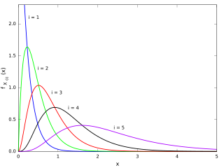
In statistics, the kth order statistic of a statistical sample is equal to its kth-smallest value. Together with rank statistics, order statistics are among the most fundamental tools in non-parametric statistics and inference.
In mathematics, summation is the addition of a sequence of numbers, called addends or summands; the result is their sum or total. Beside numbers, other types of values can be summed as well: functions, vectors, matrices, polynomials and, in general, elements of any type of mathematical objects on which an operation denoted "+" is defined.
In information theory, the typical set is a set of sequences whose probability is close to two raised to the negative power of the entropy of their source distribution. That this set has total probability close to one is a consequence of the asymptotic equipartition property (AEP) which is a kind of law of large numbers. The notion of typicality is only concerned with the probability of a sequence and not the actual sequence itself.
In numerical analysis, the quasi-Monte Carlo method is a method for numerical integration and solving some other problems using low-discrepancy sequences to achieve variance reduction. This is in contrast to the regular Monte Carlo method or Monte Carlo integration, which are based on sequences of pseudorandom numbers.
Multi-index notation is a mathematical notation that simplifies formulas used in multivariable calculus, partial differential equations and the theory of distributions, by generalising the concept of an integer index to an ordered tuple of indices.
In probability and statistics, the Dirichlet distribution (after Peter Gustav Lejeune Dirichlet), often denoted , is a family of continuous multivariate probability distributions parameterized by a vector of positive reals. It is a multivariate generalization of the beta distribution, hence its alternative name of multivariate beta distribution (MBD). Dirichlet distributions are commonly used as prior distributions in Bayesian statistics, and in fact, the Dirichlet distribution is the conjugate prior of the categorical distribution and multinomial distribution.
In information theory, Shannon's source coding theorem establishes the statistical limits to possible data compression for data whose source is an independent identically-distributed random variable, and the operational meaning of the Shannon entropy.
Sobol’ sequences (also called LPτ sequences or (t, s) sequences in base 2) are an example of quasi-random low-discrepancy sequences. They were first introduced by the Russian mathematician Ilya M. Sobol’ (Илья Меерович Соболь) in 1967.
In information theory, information dimension is an information measure for random vectors in Euclidean space, based on the normalized entropy of finely quantized versions of the random vectors. This concept was first introduced by Alfréd Rényi in 1959.
In mathematics, Doob's martingale inequality, also known as Kolmogorov’s submartingale inequality is a result in the study of stochastic processes. It gives a bound on the probability that a submartingale exceeds any given value over a given interval of time. As the name suggests, the result is usually given in the case that the process is a martingale, but the result is also valid for submartingales.
Anatoly Alexeyevich Karatsuba was a Russian mathematician working in the field of analytic number theory, p-adic numbers and Dirichlet series.
In mathematics, a quasi-analytic class of functions is a generalization of the class of real analytic functions based upon the following fact: If f is an analytic function on an interval [a,b] ⊂ R, and at some point f and all of its derivatives are zero, then f is identically zero on all of [a,b]. Quasi-analytic classes are broader classes of functions for which this statement still holds true.
In probability theory, a sub-Gaussian distribution, the distribution of a sub-Gaussian random variable, is a probability distribution with strong tail decay. More specifically, the tails of a sub-Gaussian distribution are dominated by the tails of a Gaussian. This property gives sub-Gaussian distributions their name.
References
Dick, Josef; Pillichshammer, Friedrich (2010). Digital Nets and Sequences: Discrepancy Theory and Quasi-Monte Carlo Integration. ISBN978-0-521-19159-3.
Harald Niederreiter (1992). Random Number Generation and Quasi-Monte Carlo Methods. Society for Industrial and Applied Mathematics. ISBN0-89871-295-5.
Drmota, Michael; Tichy, Robert F. (1997). Sequences, Discrepancies and Applications. Lecture Notes in Math. Vol.1651. Springer. ISBN3-540-62606-9.
Press, William H.; Flannery, Brian P.; Teukolsky, Saul A.; Vetterling, William T. (1992). Numerical Recipes in C (2nded.). Cambridge University Press. see Section 7.7 for a less technical discussion of low-discrepancy sequences. ISBN0-521-43108-5.
This page is based on this Wikipedia article Text is available under the CC BY-SA 4.0 license; additional terms may apply. Images, videos and audio are available under their respective licenses.
![Error in estimated kurtosis as a function of number of datapoints. 'Additive quasirandom' gives the maximum error when c = ([?]5 - 1)/2. 'Random' gives the average error over six runs of random numbers, where the average is taken to reduce the magnitude of the wild fluctuations Subrandom Kurtosis.gif](http://upload.wikimedia.org/wikipedia/commons/thumb/0/0e/Subrandom_Kurtosis.gif/370px-Subrandom_Kurtosis.gif)