Segment tree

Last updated
Graphic example of the structure of the segment tree. This instance is built for the segments shown at the bottom. Segment tree.svg
Graphic example of the structure of the segment tree. This instance is built for the segments shown at the bottom.

In computer science, the segment tree is a data structure used for storing information about intervals or segments. It allows querying which of the stored segments contain a given point. A similar data structure is the interval tree.

Contents

A segment tree for a set I of n intervals uses O(n log n) storage and can be built in O(n log n) time. Segment trees support searching for all the intervals that contain a query point in time O(log n + k), k being the number of retrieved intervals or segments. [1]

Applications of the segment tree are in the areas of computational geometry, geographic information systems and machine learning.

The segment tree can be generalized to higher dimension spaces.

Definition

Description

Let S be a set of intervals, or segments. Let p1, p2, ..., pm be the list of distinct interval endpoints, sorted from left to right. Consider the partitioning of the real line induced by those points. The regions of this partitioning are called elementary intervals. Thus, the elementary intervals are, from left to right:

That is, the list of elementary intervals consists of open intervals between two consecutive endpoints pi and pi+1, alternated with closed intervals consisting of a single endpoint. Single points are treated themselves as intervals because the answer to a query is not necessarily the same at the interior of an elementary interval and its endpoints. [2]

Given a set I of intervals, or segments, a segment tree T for I is structured as follows:

Construction

A segment tree from the set of segments I, can be built as follows. First, the endpoints of the intervals in I are sorted. The elementary intervals are obtained from that. Then, a balanced binary tree is built on the elementary intervals, and for each node v it is determined the interval Int(v) it represents. It remains to compute the canonical subsets for the nodes. To achieve this, the intervals in I are inserted one by one into the segment tree. An interval X = [x, x] can be inserted in a subtree rooted at T, using the following procedure: [4]

The complete construction operation takes O(n log n) time, n being the number of segments in I.

Proof
Sorting the endpoints takes O(n log n). Building a balanced binary tree from the sorted endpoints, takes linear time on n.
The insertion of an interval X = [x, x] into the tree, costs O(log n).
Proof

Visiting every node takes constant time (assuming that canonical subsets are stored in a simple data structure like a linked list). When we visit node v, we either store X at v, or Int(v) contains an endpoint of X. As proved above, an interval is stored at most twice at each level of the tree. There is also at most one node at every level whose corresponding interval contains x, and one node whose interval contains x. So, at most four nodes per level are visited. Since there are O(log n) levels, the total cost of the insertion is O(log n). [1]

Query

A query for a segment tree receives a point qx(should be one of the leaves of tree), and retrieves a list of all the segments stored which contain the point qx.

Formally stated; given a node (subtree) v and a query point qx, the query can be done using the following algorithm:

  1. Report all the intervals in I(v).
  2. If v is not a leaf:
    • If qx is in Int(left child of v) then
      • Perform a query in the left child of v.
    • If qx is in Int(right child of v) then
      • Perform a query in the right child of v.

In a segment tree that contains n intervals, those containing a given query point can be reported in O(log n + k) time, where k is the number of reported intervals.

Proof

The query algorithm visits one node per level of the tree, so O(log n) nodes in total. On the other hand, at a node v, the segments in I are reported in O(1 + kv) time, where kv is the number of intervals at node v, reported. The sum of all the kv for all nodes v visited, is k, the number of reported segments. [5]

Storage requirements

A segment tree T on a set I of n intervals uses O(n log n) storage.

Lemma   Any interval [x, x] of I is stored in the canonical set for at most two nodes at the same depth.

Proof

Let v1, v2, v3 be the three nodes at the same depth, numbered from left to right; and let p(v) be the parent node of any given node v. Suppose [x, x] is stored at v1 and v3. This means that [x, x] spans the whole interval from the left endpoint of Int(v1) to the right endpoint of Int(v3). Note that all segments at a particular level are non-overlapping and ordered from left to right: this is true by construction for the level containing the leaves, and the property is not lost when moving from any level to the one above it by combining pairs of adjacent segments. Now either parent(v2) = parent(v1), or the former is to the right of the latter (edges in the tree do not cross). In the first case, Int(parent(v2))'s leftmost point is the same as Int(v1)'s leftmost point; in the second case, Int(parent(v2))'s leftmost point is to the right of Int(parent(v1))'s rightmost point, and therefore also to the right of Int(v1)'s rightmost point. In both cases, Int(parent(v2)) begins at or to the right of Int(v1)'s leftmost point. Similar reasoning shows that Int(parent(v2)) ends at or to the left of Int(v3)'s rightmost point. Int(parent(v2)) must therefore be contained in [x, x]; hence, [x, x] will not be stored at v2.

The set I has at most 4n + 1 elementary intervals. Because T is a binary balanced tree with at most 4n + 1 leaves, its height is O(log n). Since any interval is stored at most twice at a given depth of the tree, that the total amount of storage is O(n log n). [5]


Generalization for higher dimensions

The segment tree can be generalized to higher dimension spaces, in the form of multi-level segment trees. In higher dimensional versions, the segment tree stores a collection of axis-parallel (hyper-)rectangles, and can retrieve the rectangles that contain a given query point. The structure uses O(n logdn) storage, and answers queries in O(logdn) time.

The use of fractional cascading lowers the query time bound by a logarithmic factor. The use of the interval tree on the deepest level of associated structures lowers the storage bound by a logarithmic factor. [6]

Notes

A query that asks for all the intervals containing a given point is often referred as a stabbing query. [7]

The segment tree is less efficient than the interval tree for range queries in one dimension, due to its higher storage requirement: O(n log n) against the O(n) of the interval tree. The importance of the segment tree is that the segments within each node’s canonical subset can be stored in any arbitrary manner. [7]

For n intervals whose endpoints are in a small integer range (e.g., in the range [1,...,O(n)]), optimal data structures[ which? ] exist with a linear preprocessing time and query time O(1 + k) for reporting all k intervals containing a given query point.

Another advantage of the segment tree is that it can easily be adapted to counting queries; that is, to report the number of segments containing a given point, instead of reporting the segments themselves. Instead of storing the intervals in the canonical subsets, it can simply store the number of them. Such a segment tree uses linear storage, and requires an O(log n) query time, so it is optimal. [8]

Higher dimensional versions of the interval tree and the priority search tree do not exist; that is, there is no clear extension of these structures that solves the analogous problem in higher dimensions. But the structures can be used as associated structure of segment trees. [6]

History

The segment tree was invented by Jon Bentley in 1977; in "Solutions to Klee’s rectangle problems". [7]

Related Research Articles

<span class="mw-page-title-main">Binary search algorithm</span> Search algorithm finding the position of a target value within a sorted array

In computer science, binary search, also known as half-interval search, logarithmic search, or binary chop, is a search algorithm that finds the position of a target value within a sorted array. Binary search compares the target value to the middle element of the array. If they are not equal, the half in which the target cannot lie is eliminated and the search continues on the remaining half, again taking the middle element to compare to the target value, and repeating this until the target value is found. If the search ends with the remaining half being empty, the target is not in the array.

In computer science, a red–black tree is a specialised binary search tree data structure noted for fast storage and retrieval of ordered information, and a guarantee that operations will complete within a known time. Compared to other self-balancing binary search trees, the nodes in a red-black tree hold an extra bit called "color" representing "red" and "black" which is used when re-organising the tree to ensure that it is always approximately balanced.

<span class="mw-page-title-main">Treap</span>

In computer science, the treap and the randomized binary search tree are two closely related forms of binary search tree data structures that maintain a dynamic set of ordered keys and allow binary searches among the keys. After any sequence of insertions and deletions of keys, the shape of the tree is a random variable with the same probability distribution as a random binary tree; in particular, with high probability its height is proportional to the logarithm of the number of keys, so that each search, insertion, or deletion operation takes logarithmic time to perform.

<span class="mw-page-title-main">Quadtree</span> Tree data structure in which each internal node has exactly four children, to partition a 2D area

A quadtree is a tree data structure in which each internal node has exactly four children. Quadtrees are the two-dimensional analog of octrees and are most often used to partition a two-dimensional space by recursively subdividing it into four quadrants or regions. The data associated with a leaf cell varies by application, but the leaf cell represents a "unit of interesting spatial information".

In computing, a persistent data structure or not ephemeral data structure is a data structure that always preserves the previous version of itself when it is modified. Such data structures are effectively immutable, as their operations do not (visibly) update the structure in-place, but instead always yield a new updated structure. The term was introduced in Driscoll, Sarnak, Sleator, and Tarjan's 1986 article.

In computer science, a disjoint-set data structure, also called a union–find data structure or merge–find set, is a data structure that stores a collection of disjoint (non-overlapping) sets. Equivalently, it stores a partition of a set into disjoint subsets. It provides operations for adding new sets, merging sets, and finding a representative member of a set. The last operation makes it possible to find out efficiently if any two elements are in the same or different sets.

<span class="mw-page-title-main">Rope (data structure)</span> Data structure for storing strings

In computer programming, a rope, or cord, is a data structure composed of smaller strings that is used to efficiently store and manipulate a very long string. For example, a text editing program may use a rope to represent the text being edited, so that operations such as insertion, deletion, and random access can be done efficiently.

A B+ tree is an m-ary tree with a variable but often large number of children per node. A B+ tree consists of a root, internal nodes and leaves. The root may be either a leaf or a node with two or more children.

In computer science, an interval tree is a tree data structure to hold intervals. Specifically, it allows one to efficiently find all intervals that overlap with any given interval or point. It is often used for windowing queries, for instance, to find all roads on a computerized map inside a rectangular viewport, or to find all visible elements inside a three-dimensional scene. A similar data structure is the segment tree.

<i>k</i>-d tree Multidimensional search tree for points in k dimensional space

In computer science, a k-d tree is a space-partitioning data structure for organizing points in a k-dimensional space. K-dimensional is that which concerns exactly k orthogonal axes or a space of any number of dimensions. k-d trees are a useful data structure for several applications, such as:

In graph theory and computer science, the lowest common ancestor (LCA) of two nodes v and w in a tree or directed acyclic graph (DAG) T is the lowest node that has both v and w as descendants, where we define each node to be a descendant of itself.

A link/cut tree is a data structure for representing a forest, a set of rooted trees, and offers the following operations:

In computer science, a range tree is an ordered tree data structure to hold a list of points. It allows all points within a given range to be reported efficiently, and is typically used in two or higher dimensions. Range trees were introduced by Jon Louis Bentley in 1979. Similar data structures were discovered independently by Lueker, Lee and Wong, and Willard. The range tree is an alternative to the k-d tree. Compared to k-d trees, range trees offer faster query times of but worse storage of , where n is the number of points stored in the tree, d is the dimension of each point and k is the number of points reported by a given query.

<span class="mw-page-title-main">Cartesian tree</span> Binary tree derived from a sequence of numbers

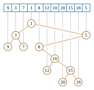
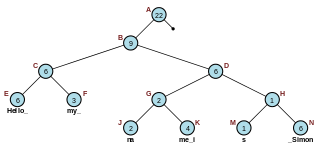
In computer science, a Cartesian tree is a binary tree derived from a sequence of distinct numbers. To construct the Cartesian tree, set its root to be the minimum number in the sequence, and recursively construct its left and right subtrees from the subsequences before and after this number. It is uniquely defined as a min-heap whose symmetric (in-order) traversal returns the original sequence.

In computational geometry, the Bentley–Ottmann algorithm is a sweep line algorithm for listing all crossings in a set of line segments, i.e. it finds the intersection points of line segments. It extends the Shamos–Hoey algorithm, a similar previous algorithm for testing whether or not a set of line segments has any crossings. For an input consisting of line segments with crossings, the Bentley–Ottmann algorithm takes time . In cases where , this is an improvement on a naïve algorithm that tests every pair of segments, which takes .

<span class="mw-page-title-main">Fenwick tree</span> Data structure

A Fenwick tree or binary indexed tree(BIT) is a data structure that can efficiently update values and calculate prefix sums in an array of values.

In computer science, a double-ended priority queue (DEPQ) or double-ended heap is a data structure similar to a priority queue or heap, but allows for efficient removal of both the maximum and minimum, according to some ordering on the keys (items) stored in the structure. Every element in a DEPQ has a priority or value. In a DEPQ, it is possible to remove the elements in both ascending as well as descending order.

In computer science, an x-fast trie is a data structure for storing integers from a bounded domain. It supports exact and predecessor or successor queries in time O(log log M), using O(n log M) space, where n is the number of stored values and M is the maximum value in the domain. The structure was proposed by Dan Willard in 1982, along with the more complicated y-fast trie, as a way to improve the space usage of van Emde Boas trees, while retaining the O(log log M) query time.

In computer science, the range query problem consists of efficiently answering several queries regarding a given interval of elements within an array. For example, a common task, known as range minimum query, is finding the smallest value inside a given range within a list of numbers.

<span class="mw-page-title-main">Finger search</span>

In computer science, a finger search on a data structure is an extension of any search operation that structure supports, where a reference (finger) to an element in the data structure is given along with the query. While the search time for an element is most frequently expressed as a function of the number of elements in a data structure, finger search times are a function of the distance between the element and the finger.

References

  1. 1 2 ( de Berg et al. 2000 , p. 227)
  2. ( de Berg et al. 2000 , p. 224)
  3. ( de Berg et al. 2000 , pp. 225–226)
  4. ( de Berg et al. 2000 , pp. 226–227)
  5. 1 2 ( de Berg et al. 2000 , p. 226)
  6. 1 2 ( de Berg et al. 2000 , p. 230)
  7. 1 2 3 ( de Berg et al. 2000 , p. 229)
  8. ( de Berg et al. 2000 , pp. 229–230)

Sources cited