In mathematics and statistics, the arithmetic mean or arithmetic average, or just the mean or the average, is the sum of a collection of numbers divided by the count of numbers in the collection. The collection is often a set of results of an experiment or an observational study, or frequently a set of results from a survey. The term "arithmetic mean" is preferred in some contexts in mathematics and statistics, because it helps distinguish it from other means, such as the geometric mean and the harmonic mean.

In statistics and probability theory, the median is the value separating the higher half from the lower half of a data sample, a population, or a probability distribution. For a data set, it may be thought of as "the middle" value. The basic feature of the median in describing data compared to the mean is that it is not skewed by a small proportion of extremely large or small values, and therefore provides a better representation of a "typical" value. Median income, for example, may be a better way to suggest what a "typical" income is, because income distribution can be very skewed. The median is of central importance in robust statistics, as it is the most resistant statistic, having a breakdown point of 50%: so long as no more than half the data are contaminated, the median is not an arbitrarily large or small result.

In statistics, a normal distribution is a type of continuous probability distribution for a real-valued random variable. The general form of its probability density function is

In statistics, the standard deviation is a measure of the amount of variation or dispersion of a set of values. A low standard deviation indicates that the values tend to be close to the mean of the set, while a high standard deviation indicates that the values are spread out over a wider range.
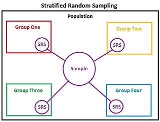
In statistics, stratified sampling is a method of sampling from a population which can be partitioned into subpopulations.

In probability theory and statistics, skewness is a measure of the asymmetry of the probability distribution of a real-valued random variable about its mean. The skewness value can be positive, zero, negative, or undefined.

In probability theory and statistics, variance is the expectation of the squared deviation of a random variable from its population mean or sample mean. Variance is a measure of dispersion, meaning it is a measure of how far a set of numbers is spread out from their average value. Variance has a central role in statistics, where some ideas that use it include descriptive statistics, statistical inference, hypothesis testing, goodness of fit, and Monte Carlo sampling. Variance is an important tool in the sciences, where statistical analysis of data is common. The variance is the square of the standard deviation, the second central moment of a distribution, and the covariance of the random variable with itself, and it is often represented by , , , , or .
The weighted arithmetic mean is similar to an ordinary arithmetic mean, except that instead of each of the data points contributing equally to the final average, some data points contribute more than others. The notion of weighted mean plays a role in descriptive statistics and also occurs in a more general form in several other areas of mathematics.

In probability theory, a log-normaldistribution is a continuous probability distribution of a random variable whose logarithm is normally distributed. Thus, if the random variable X is log-normally distributed, then Y = ln(X) has a normal distribution. Equivalently, if Y has a normal distribution, then the exponential function of Y, X = exp(Y), has a log-normal distribution. A random variable which is log-normally distributed takes only positive real values. It is a convenient and useful model for measurements in exact and engineering sciences, as well as medicine, economics and other topics.
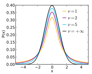
In probability and statistics, Student's t-distribution is any member of a family of continuous probability distributions that arise when estimating the mean of a normally distributed population in situations where the sample size is small and the population's standard deviation is unknown. It was developed by English statistician William Sealy Gosset under the pseudonym "Student".
In probability theory, Chebyshev's inequality guarantees that, for a wide class of probability distributions, no more than a certain fraction of values can be more than a certain distance from the mean. Specifically, no more than 1/k2 of the distribution's values can be k or more standard deviations away from the mean. The rule is often called Chebyshev's theorem, about the range of standard deviations around the mean, in statistics. The inequality has great utility because it can be applied to any probability distribution in which the mean and variance are defined. For example, it can be used to prove the weak law of large numbers.
The standard error (SE) of a statistic is the standard deviation of its sampling distribution or an estimate of that standard deviation. If the statistic is the sample mean, it is called the standard error of the mean (SEM).

The Bloch MB.170 and its derivatives were French reconnaissance bombers designed and built shortly before the Second World War. They were the best aircraft of this type available to the Armée de l'Air at the outbreak of the war, with speed, altitude and manoeuvrability that allowed them to evade interception by the German fighters. Although the aircraft could have been in service by 1937, debate over what role to give the aircraft delayed deliveries until 1940.
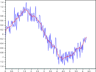
In statistics, a moving average is a calculation to analyze data points by creating a series of averages of different subsets of the full data set. It is also called a moving mean (MM) or rolling mean and is a type of finite impulse response filter. Variations include: simple, cumulative, or weighted forms.
In probability theory and statistics, the coefficient of variation (CV), also known as relative standard deviation (RSD), is a standardized measure of dispersion of a probability distribution or frequency distribution. It is often expressed as a percentage, and is defined as the ratio of the standard deviation to the mean . The CV or RSD is widely used in analytical chemistry to express the precision and repeatability of an assay. It is also commonly used in fields such as engineering or physics when doing quality assurance studies and ANOVA gauge R&R, by economists and investors in economic models, and in neuroscience.
In estimation theory and decision theory, a Bayes estimator or a Bayes action is an estimator or decision rule that minimizes the posterior expected value of a loss function. Equivalently, it maximizes the posterior expectation of a utility function. An alternative way of formulating an estimator within Bayesian statistics is maximum a posteriori estimation.
Squared deviations from the mean (SDM) are involved in various calculations. In probability theory and statistics, the definition of variance is either the expected value of the SDM or its average value. Computations for analysis of variance involve the partitioning of a sum of SDM.
In statistics and in particular statistical theory, unbiased estimation of a standard deviation is the calculation from a statistical sample of an estimated value of the standard deviation of a population of values, in such a way that the expected value of the calculation equals the true value. Except in some important situations, outlined later, the task has little relevance to applications of statistics since its need is avoided by standard procedures, such as the use of significance tests and confidence intervals, or by using Bayesian analysis.
Kuznyechik is a symmetric block cipher. It has a block size of 128 bits and key length of 256 bits. It is defined in the National Standard of the Russian Federation GOST R 34.12-2015 and also in RFC 7801.


