
Pell's equation, also called the Pell–Fermat equation, is any Diophantine equation of the form where n is a given positive nonsquare integer, and integer solutions are sought for x and y. In Cartesian coordinates, the equation is represented by a hyperbola; solutions occur wherever the curve passes through a point whose x and y coordinates are both integers, such as the trivial solution with x = 1 and y = 0. Joseph Louis Lagrange proved that, as long as n is not a perfect square, Pell's equation has infinitely many distinct integer solutions. These solutions may be used to accurately approximate the square root of n by rational numbers of the form x/y.

In mathematics, the slope or gradient of a line is a number that describes both the direction and the steepness of the line. Slope is often denoted by the letter m; there is no clear answer to the question why the letter m is used for slope, but its earliest use in English appears in O'Brien (1844) who wrote the equation of a straight line as "y = mx + b" and it can also be found in Todhunter (1888) who wrote it as "y = mx + c".

In geometry, the tangent line (or simply tangent) to a plane curve at a given point is, intuitively, the straight line that "just touches" the curve at that point. Leibniz defined it as the line through a pair of infinitely close points on the curve. More precisely, a straight line is tangent to the curve y = f(x) at a point x = c if the line passes through the point (c, f(c)) on the curve and has slope f'(c), where f' is the derivative of f. A similar definition applies to space curves and curves in n-dimensional Euclidean space.

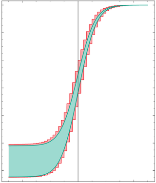
In probability theory, a probability density function (PDF), density function, or density of an absolutely continuous random variable, is a function whose value at any given sample in the sample space can be interpreted as providing a relative likelihood that the value of the random variable would be equal to that sample. Probability density is the probability per unit length, in other words, while the absolute likelihood for a continuous random variable to take on any particular value is 0, the value of the PDF at two different samples can be used to infer, in any particular draw of the random variable, how much more likely it is that the random variable would be close to one sample compared to the other sample.
Bresenham's line algorithm is a line drawing algorithm that determines the points of an n-dimensional raster that should be selected in order to form a close approximation to a straight line between two points. It is commonly used to draw line primitives in a bitmap image, as it uses only integer addition, subtraction, and bit shifting, all of which are very cheap operations in historically common computer architectures. It is an incremental error algorithm, and one of the earliest algorithms developed in the field of computer graphics. An extension to the original algorithm called the midpoint circle algorithm may be used for drawing circles.
In mathematics, a Diophantine equation is an equation of the form P(x1, ..., xj, y1, ..., yk) = 0 (usually abbreviated P(x, y) = 0) where P(x, y) is a polynomial with integer coefficients, where x1, ..., xj indicate parameters and y1, ..., yk indicate unknowns.

In computer graphics, a line drawing algorithm is an algorithm for approximating a line segment on discrete graphical media, such as pixel-based displays and printers. On such media, line drawing requires an approximation. Basic algorithms rasterize lines in one color. A better representation with multiple color gradations requires an advanced process, spatial anti-aliasing.
The Lenstra elliptic-curve factorization or the elliptic-curve factorization method (ECM) is a fast, sub-exponential running time, algorithm for integer factorization, which employs elliptic curves. For general-purpose factoring, ECM is the third-fastest known factoring method. The second-fastest is the multiple polynomial quadratic sieve, and the fastest is the general number field sieve. The Lenstra elliptic-curve factorization is named after Hendrik Lenstra.
In numerical analysis, polynomial interpolation is the interpolation of a given bivariate data set by the polynomial of lowest possible degree that passes through the points of the dataset.
In the mathematical field of numerical analysis, a Newton polynomial, named after its inventor Isaac Newton, is an interpolation polynomial for a given set of data points. The Newton polynomial is sometimes called Newton's divided differences interpolation polynomial because the coefficients of the polynomial are calculated using Newton's divided differences method.
In the mathematical field of numerical analysis, spline interpolation is a form of interpolation where the interpolant is a special type of piecewise polynomial called a spline. That is, instead of fitting a single, high-degree polynomial to all of the values at once, spline interpolation fits low-degree polynomials to small subsets of the values, for example, fitting nine cubic polynomials between each of the pairs of ten points, instead of fitting a single degree-nine polynomial to all of them. Spline interpolation is often preferred over polynomial interpolation because the interpolation error can be made small even when using low-degree polynomials for the spline. Spline interpolation also avoids the problem of Runge's phenomenon, in which oscillation can occur between points when interpolating using high-degree polynomials.

In mathematics, bilinear interpolation is a method for interpolating functions of two variables using repeated linear interpolation. It is usually applied to functions sampled on a 2D rectilinear grid, though it can be generalized to functions defined on the vertices of arbitrary convex quadrilaterals.
In mathematics, the rearrangement inequality states that for every choice of real numbers
In mathematics, divided differences is an algorithm, historically used for computing tables of logarithms and trigonometric functions. Charles Babbage's difference engine, an early mechanical calculator, was designed to use this algorithm in its operation.
Particle filters, or sequential Monte Carlo methods, are a set of Monte Carlo algorithms used to find approximate solutions for filtering problems for nonlinear state-space systems, such as signal processing and Bayesian statistical inference. The filtering problem consists of estimating the internal states in dynamical systems when partial observations are made and random perturbations are present in the sensors as well as in the dynamical system. The objective is to compute the posterior distributions of the states of a Markov process, given the noisy and partial observations. The term "particle filters" was first coined in 1996 by Pierre Del Moral about mean-field interacting particle methods used in fluid mechanics since the beginning of the 1960s. The term "Sequential Monte Carlo" was coined by Jun S. Liu and Rong Chen in 1998.
Muller's method is a root-finding algorithm, a numerical method for solving equations of the form f(x) = 0. It was first presented by David E. Muller in 1956.
In computer graphics, the Liang–Barsky algorithm is a line clipping algorithm. The Liang–Barsky algorithm uses the parametric equation of a line and inequalities describing the range of the clipping window to determine the intersections between the line and the clip window. With these intersections it knows which portion of the line should be drawn. So this algorithm is significantly more efficient than Cohen–Sutherland. The idea of the Liang–Barsky clipping algorithm is to do as much testing as possible before computing line intersections.
Interval arithmetic is a mathematical technique used to mitigate rounding and measurement errors in mathematical computation by computing function bounds. Numerical methods involving interval arithmetic can guarantee relatively reliable and mathematically correct results. Instead of representing a value as a single number, interval arithmetic or interval mathematics represents each value as a range of possibilities.
In geometry, the Hessian curve is a plane curve similar to folium of Descartes. It is named after the German mathematician Otto Hesse. This curve was suggested for application in elliptic curve cryptography, because arithmetic in this curve representation is faster and needs less memory than arithmetic in standard Weierstrass form.
In the mathematical field of numerical analysis, monotone cubic interpolation is a variant of cubic interpolation that preserves monotonicity of the data set being interpolated.


