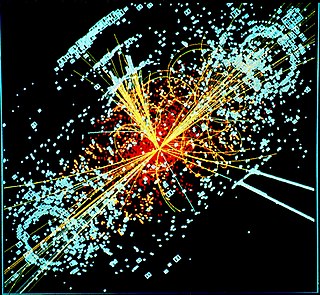
In physics, the CHSH inequality can be used in the proof of Bell's theorem, which states that certain consequences of entanglement in quantum mechanics cannot be reproduced by local hidden-variable theories. Experimental verification of the inequality being violated is seen as confirmation that nature cannot be described by such theories. CHSH stands for John Clauser, Michael Horne, Abner Shimony, and Richard Holt, who described it in a much-cited paper published in 1969. They derived the CHSH inequality, which, as with John Stewart Bell's original inequality, is a constraint on the statistical occurrence of "coincidences" in a Bell test which is necessarily true if there exist underlying local hidden variables, an assumption that is sometimes termed local realism. In practice, the inequality is routinely violated by modern experiments in quantum mechanics.
Linear elasticity is a mathematical model of how solid objects deform and become internally stressed due to prescribed loading conditions. It is a simplification of the more general nonlinear theory of elasticity and a branch of continuum mechanics.
In physics, a partition function describes the statistical properties of a system in thermodynamic equilibrium. Partition functions are functions of the thermodynamic state variables, such as the temperature and volume. Most of the aggregate thermodynamic variables of the system, such as the total energy, free energy, entropy, and pressure, can be expressed in terms of the partition function or its derivatives. The partition function is dimensionless.
In mathematics, Schur's lemma is an elementary but extremely useful statement in representation theory of groups and algebras. In the group case it says that if M and N are two finite-dimensional irreducible representations of a group G and φ is a linear map from M to N that commutes with the action of the group, then either φ is invertible, or φ = 0. An important special case occurs when M = N, i.e. φ is a self-map; in particular, any element of the center of a group must act as a scalar operator on M. The lemma is named after Issai Schur who used it to prove the Schur orthogonality relations and develop the basics of the representation theory of finite groups. Schur's lemma admits generalisations to Lie groups and Lie algebras, the most common of which are due to Jacques Dixmier and Daniel Quillen.
In physics, mathematics and statistics, scale invariance is a feature of objects or laws that do not change if scales of length, energy, or other variables, are multiplied by a common factor, and thus represent a universality.

In probability and statistics, the Yule–Simon distribution is a discrete probability distribution named after Udny Yule and Herbert A. Simon. Simon originally called it the Yule distribution.
In mathematics, the von Mangoldt function is an arithmetic function named after German mathematician Hans von Mangoldt. It is an example of an important arithmetic function that is neither multiplicative nor additive.
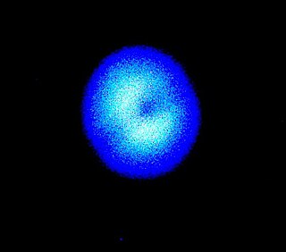
In optics, the Fresnel diffraction equation for near-field diffraction is an approximation of the Kirchhoff–Fresnel diffraction that can be applied to the propagation of waves in the near field. It is used to calculate the diffraction pattern created by waves passing through an aperture or around an object, when viewed from relatively close to the object. In contrast the diffraction pattern in the far field region is given by the Fraunhofer diffraction equation.
Bayesian linear regression is a type of conditional modeling in which the mean of one variable is described by a linear combination of other variables, with the goal of obtaining the posterior probability of the regression coefficients and ultimately allowing the out-of-sample prediction of the regressandconditional on observed values of the regressors. The simplest and most widely used version of this model is the normal linear model, in which given is distributed Gaussian. In this model, and under a particular choice of prior probabilities for the parameters—so-called conjugate priors—the posterior can be found analytically. With more arbitrarily chosen priors, the posteriors generally have to be approximated.
A ratio distribution is a probability distribution constructed as the distribution of the ratio of random variables having two other known distributions. Given two random variables X and Y, the distribution of the random variable Z that is formed as the ratio Z = X/Y is a ratio distribution.
In probability and statistics, the Tweedie distributions are a family of probability distributions which include the purely continuous normal, gamma and inverse Gaussian distributions, the purely discrete scaled Poisson distribution, and the class of compound Poisson–gamma distributions which have positive mass at zero, but are otherwise continuous. Tweedie distributions are a special case of exponential dispersion models and are often used as distributions for generalized linear models.
The Heckman correction is a statistical technique to correct bias from non-randomly selected samples or otherwise incidentally truncated dependent variables, a pervasive issue in quantitative social sciences when using observational data. Conceptually, this is achieved by explicitly modelling the individual sampling probability of each observation together with the conditional expectation of the dependent variable. The resulting likelihood function is mathematically similar to the tobit model for censored dependent variables, a connection first drawn by James Heckman in 1974. Heckman also developed a two-step control function approach to estimate this model, which avoids the computational burden of having to estimate both equations jointly, albeit at the cost of inefficiency. Heckman received the Nobel Memorial Prize in Economic Sciences in 2000 for his work in this field.
In mathematics, the spectral theory of ordinary differential equations is the part of spectral theory concerned with the determination of the spectrum and eigenfunction expansion associated with a linear ordinary differential equation. In his dissertation, Hermann Weyl generalized the classical Sturm–Liouville theory on a finite closed interval to second order differential operators with singularities at the endpoints of the interval, possibly semi-infinite or infinite. Unlike the classical case, the spectrum may no longer consist of just a countable set of eigenvalues, but may also contain a continuous part. In this case the eigenfunction expansion involves an integral over the continuous part with respect to a spectral measure, given by the Titchmarsh–Kodaira formula. The theory was put in its final simplified form for singular differential equations of even degree by Kodaira and others, using von Neumann's spectral theorem. It has had important applications in quantum mechanics, operator theory and harmonic analysis on semisimple Lie groups.
In mathematics, log-polar coordinates is a coordinate system in two dimensions, where a point is identified by two numbers, one for the logarithm of the distance to a certain point, and one for an angle. Log-polar coordinates are closely connected to polar coordinates, which are usually used to describe domains in the plane with some sort of rotational symmetry. In areas like harmonic and complex analysis, the log-polar coordinates are more canonical than polar coordinates.
In optics, the Fraunhofer diffraction equation is used to model the diffraction of waves when the diffraction pattern is viewed at a long distance from the diffracting object, and also when it is viewed at the focal plane of an imaging lens.
The theory of causal fermion systems is an approach to describe fundamental physics. It provides a unification of the weak, the strong and the electromagnetic forces with gravity at the level of classical field theory. Moreover, it gives quantum mechanics as a limiting case and has revealed close connections to quantum field theory. Therefore, it is a candidate for a unified physical theory. Instead of introducing physical objects on a preexisting spacetime manifold, the general concept is to derive spacetime as well as all the objects therein as secondary objects from the structures of an underlying causal fermion system. This concept also makes it possible to generalize notions of differential geometry to the non-smooth setting. In particular, one can describe situations when spacetime no longer has a manifold structure on the microscopic scale. As a result, the theory of causal fermion systems is a proposal for quantum geometry and an approach to quantum gravity.
The generalized functional linear model (GFLM) is an extension of the generalized linear model (GLM) that allows one to regress univariate responses of various types on functional predictors, which are mostly random trajectories generated by a square-integrable stochastic processes. Similarly to GLM, a link function relates the expected value of the response variable to a linear predictor, which in case of GFLM is obtained by forming the scalar product of the random predictor function with a smooth parameter function . Functional Linear Regression, Functional Poisson Regression and Functional Binomial Regression, with the important Functional Logistic Regression included, are special cases of GFLM. Applications of GFLM include classification and discrimination of stochastic processes and functional data.
Regularized least squares (RLS) is a family of methods for solving the least-squares problem while using regularization to further constrain the resulting solution.
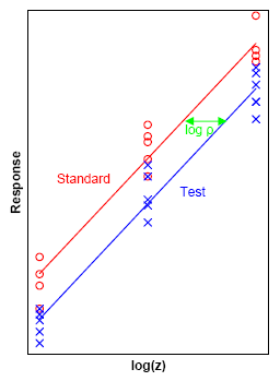
Response modeling methodology (RMM) is a general platform for statistical modeling of a linear/nonlinear relationship between a response variable (dependent variable) and a linear predictor (a linear combination of predictors/effects/factors/independent variables), often denoted the linear predictor function. It is generally assumed that the modeled relationship is monotone convex (delivering monotone convex function) or monotone concave (delivering monotone concave function). However, many non-monotone functions, like the quadratic equation, are special cases of the general model.

Batch normalization is a method used to make training of artificial neural networks faster and more stable through normalization of the layers' inputs by re-centering and re-scaling. It was proposed by Sergey Ioffe and Christian Szegedy in 2015.