In statistics, a central tendency is a central or typical value for a probability distribution.

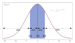
In descriptive statistics, the interquartile range (IQR) is a measure of statistical dispersion, which is the spread of the data. The IQR may also be called the midspread, middle 50%, fourth spread, or H‑spread. It is defined as the difference between the 75th and 25th percentiles of the data. To calculate the IQR, the data set is divided into quartiles, or four rank-ordered even parts via linear interpolation. These quartiles are denoted by Q1 (also called the lower quartile), Q2 (the median), and Q3 (also called the upper quartile). The lower quartile corresponds with the 25th percentile and the upper quartile corresponds with the 75th percentile, so IQR = Q3 − Q1.

In statistics and probability theory, the median is the value separating the higher half from the lower half of a data sample, a population, or a probability distribution. For a data set, it may be thought of as "the middle" value. The basic feature of the median in describing data compared to the mean is that it is not skewed by a small proportion of extremely large or small values, and therefore provides a better representation of the center. Median income, for example, may be a better way to describe the center of the income distribution because increases in the largest incomes alone have no effect on the median. For this reason, the median is of central importance in robust statistics.
A mean is a numeric quantity representing the center of a collection of numbers and is intermediate to the extreme values of a set of numbers. There are several kinds of means in mathematics, especially in statistics. Each mean serves to summarize a given group of data, often to better understand the overall value of a given data set.
In statistics, quartiles are a type of quantiles which divide the number of data points into four parts, or quarters, of more-or-less equal size. The data must be ordered from smallest to largest to compute quartiles; as such, quartiles are a form of order statistic. The three quartiles, resulting in four data divisions, are as follows:
In statistics and probability, quantiles are cut points dividing the range of a probability distribution into continuous intervals with equal probabilities, or dividing the observations in a sample in the same way. There is one fewer quantile than the number of groups created. Common quantiles have special names, such as quartiles, deciles, and percentiles. The groups created are termed halves, thirds, quarters, etc., though sometimes the terms for the quantile are used for the groups created, rather than for the cut points.

In descriptive statistics, summary statistics are used to summarize a set of observations, in order to communicate the largest amount of information as simply as possible. Statisticians commonly try to describe the observations in
The interquartile mean (IQM) is a statistical measure of central tendency based on the truncated mean of the interquartile range. The IQM is very similar to the scoring method used in sports that are evaluated by a panel of judges: discard the lowest and the highest scores; calculate the mean value of the remaining scores.
In descriptive statistics, a box plot or boxplot is a method for graphically demonstrating the locality, spread and skewness groups of numerical data through their quartiles. In addition to the box on a box plot, there can be lines extending from the box indicating variability outside the upper and lower quartiles, thus, the plot is also called the box-and-whisker plot and the box-and-whisker diagram. Outliers that differ significantly from the rest of the dataset may be plotted as individual points beyond the whiskers on the box-plot. Box plots are non-parametric: they display variation in samples of a statistical population without making any assumptions of the underlying statistical distribution. The spacings in each subsection of the box-plot indicate the degree of dispersion (spread) and skewness of the data, which are usually described using the five-number summary. In addition, the box-plot allows one to visually estimate various L-estimators, notably the interquartile range, midhinge, range, mid-range, and trimean. Box plots can be drawn either horizontally or vertically.
In statistics, a k-thpercentile, also known as percentile score or centile, is a score below which a given percentage k of scores in its frequency distribution falls or a score at or below which a given percentage falls. Percentiles are expressed in the same unit of measurement as the input scores, not in percent; for example, if the scores refer to human weight, the corresponding percentiles will be expressed in kilograms or pounds. In the limit of an infinite sample size, the percentile approximates the percentile function, the inverse of the cumulative distribution function.
A truncated mean or trimmed mean is a statistical measure of central tendency, much like the mean and median. It involves the calculation of the mean after discarding given parts of a probability distribution or sample at the high and low end, and typically discarding an equal amount of both. This number of points to be discarded is usually given as a percentage of the total number of points, but may also be given as a fixed number of points.
This glossary of statistics and probability is a list of definitions of terms and concepts used in the mathematical sciences of statistics and probability, their sub-disciplines, and related fields. For additional related terms, see Glossary of mathematics and Glossary of experimental design.
In statistics the trimean (TM), or Tukey's trimean, is a measure of a probability distribution's location defined as a weighted average of the distribution's median and its two quartiles:
In statistics, the median absolute deviation (MAD) is a robust measure of the variability of a univariate sample of quantitative data. It can also refer to the population parameter that is estimated by the MAD calculated from a sample.
In statistics, the midhinge is the average of the first and third quartiles and is thus a measure of location. Equivalently, it is the 25% trimmed mid-range or 25% midsummary; it is an L-estimator.
In statistics, an L-estimator is an estimator which is a linear combination of order statistics of the measurements. This can be as little as a single point, as in the median, or as many as all points, as in the mean.
In descriptive statistics, the seven-number summary is a collection of seven summary statistics, and is an extension of the five-number summary. There are three similar, common forms.
In statistics, a trimmed estimator is an estimator derived from another estimator by excluding some of the extreme values, a process called truncation. This is generally done to obtain a more robust statistic, and the extreme values are considered outliers. Trimmed estimators also often have higher efficiency for mixture distributions and heavy-tailed distributions than the corresponding untrimmed estimator, at the cost of lower efficiency for other distributions, such as the normal distribution.
In statistics, the interdecile range is the difference between the first and the ninth deciles. The interdecile range is a measure of statistical dispersion of the values in a set of data, similar to the range and the interquartile range, and can be computed from the (non-parametric) seven-number summary.
In statistics, robust measures of scale are methods that quantify the statistical dispersion in a sample of numerical data while resisting outliers. The most common such robust statistics are the interquartile range (IQR) and the median absolute deviation (MAD). These are contrasted with conventional or non-robust measures of scale, such as sample standard deviation, which are greatly influenced by outliers.
