McKay's approximation for the coefficient of variation

Last updated April 27, 2023

In statistics, McKay's approximation of the coefficient of variation is a statistic based on a sample from a normally distributed population. It was introduced in 1932 by A. T. McKay.^[1] Statistical methods for the coefficient of variation often utilizes McKay's approximation.^[2]^[3]^[4]^[5]

Let $x_{i}$ , $i=1,2,\ldots ,n$ be $n$ independent observations from a $N(\mu ,\sigma ^{2})$ normal distribution. The population coefficient of variation is $c_{v}=\sigma /\mu$ . Let ${\bar {x}}$ and $s\,$ denote the sample mean and the sample standard deviation, respectively. Then ${\hat {c}}_{v}=s/{\bar {x}}$ is the sample coefficient of variation. McKay's approximation is

K=\left(1+{\frac {1}{c_{v}^{2}}}\right)\ {\frac {(n-1)\ {\hat {c}}_{v}^{2}}{1+(n-1)\ {\hat {c}}_{v}^{2}/n}}

Note that in this expression, the first factor includes the population coefficient of variation, which is usually unknown. When $c_{v}$ is smaller than 1/3, then $K$ is approximately chi-square distributed with $n-1$ degrees of freedom. In the original article by McKay, the expression for $K$ looks slightly different, since McKay defined $\sigma ^{2}$ with denominator $n$ instead of $n-1$ . McKay's approximation, $K$ , for the coefficient of variation is approximately chi-square distributed, but exactly noncentral beta distributed .^[6]

Related Research Articles

In statistics, a normal distribution or Gaussian distribution is a type of continuous probability distribution for a real-valued random variable. The general form of its probability density function is

In statistics, the standard deviation is a measure of the amount of variation or dispersion of a set of values. A low standard deviation indicates that the values tend to be close to the mean of the set, while a high standard deviation indicates that the values are spread out over a wider range.

<span class="mw-page-title-main">Skewness</span> Measure of the asymmetry of random variables

In probability theory and statistics, skewness is a measure of the asymmetry of the probability distribution of a real-valued random variable about its mean. The skewness value can be positive, zero, negative, or undefined.

In probability theory, the central limit theorem (CLT) establishes that, in many situations, for identically distributed independent samples, the standardized sample mean tends towards the standard normal distribution even if the original variables themselves are not normally distributed.

<span class="mw-page-title-main">Log-normal distribution</span> Probability distribution

In probability theory, a log-normal (or lognormal) distribution is a continuous probability distribution of a random variable whose logarithm is normally distributed. Thus, if the random variable $X$ is log-normally distributed, then $Y = ln(X)$ has a normal distribution. Equivalently, if $Y$ has a normal distribution, then the exponential function of $Y$ , $X = exp(Y)$ , has a log-normal distribution. A random variable which is log-normally distributed takes only positive real values. It is a convenient and useful model for measurements in exact and engineering sciences, as well as medicine, economics and other topics (e.g., energies, concentrations, lengths, prices of financial instruments, and other metrics).

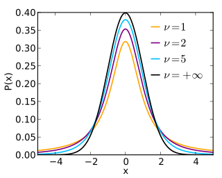
In probability and statistics, Student's t-distribution is any member of a family of continuous probability distributions that arise when estimating the mean of a normally distributed population in situations where the sample size is small and the population's standard deviation is unknown. It was developed by English statistician William Sealy Gosset under the pseudonym "Student".

In statistics, the Pearson correlation coefficient ― also known as Pearson's r, the Pearson product-moment correlation coefficient (PPMCC), the bivariate correlation, or colloquially simply as the correlation coefficient ― is a measure of linear correlation between two sets of data. It is the ratio between the covariance of two variables and the product of their standard deviations; thus, it is essentially a normalized measurement of the covariance, such that the result always has a value between −1 and 1. As with covariance itself, the measure can only reflect a linear correlation of variables, and ignores many other types of relationships or correlations. As a simple example, one would expect the age and height of a sample of teenagers from a high school to have a Pearson correlation coefficient significantly greater than 0, but less than 1.

A Z-test is any statistical test for which the distribution of the test statistic under the null hypothesis can be approximated by a normal distribution. Z-tests test the mean of a distribution. For each significance level in the confidence interval, the Z-test has a single critical value which makes it more convenient than the Student's t-test whose critical values are defined by the sample size. Both the Z-test and Student's t-test have similarities in that they both help determine the significance of a set of data. However, the z-test is rarely used in practice because the population deviation is difficult to determine.

In statistical inference, specifically predictive inference, a prediction interval is an estimate of an interval in which a future observation will fall, with a certain probability, given what has already been observed. Prediction intervals are often used in regression analysis.

In statistics, propagation of uncertainty is the effect of variables' uncertainties on the uncertainty of a function based on them. When the variables are the values of experimental measurements they have uncertainties due to measurement limitations which propagate due to the combination of variables in the function.

In probability theory and statistics, the coefficient of variation (CV), also known as relative standard deviation (RSD), is a standardized measure of dispersion of a probability distribution or frequency distribution. It is often expressed as a percentage, and is defined as the ratio of the standard deviation $to the mean . The CV or RSD is widely used in analytical chemistry to express the precision and repeatability of an assay. It is also commonly used in fields such as engineering or physics when doing quality assurance studies and ANOVA gauge R&R, by economists and investors in economic models, and in neuroscience.$

<span class="mw-page-title-main">Multimodal distribution</span> Probability distribution whose density has two or more distinct local maxima

In statistics, a multimodaldistribution is a probability distribution with more than one mode. These appear as distinct peaks in the probability density function, as shown in Figures 1 and 2. Categorical, continuous, and discrete data can all form multimodal distributions. Among univariate analyses, multimodal distributions are commonly bimodal.

In Bayesian statistics, a maximum a posteriori probability (MAP) estimate is an estimate of an unknown quantity, that equals the mode of the posterior distribution. The MAP can be used to obtain a point estimate of an unobserved quantity on the basis of empirical data. It is closely related to the method of maximum likelihood (ML) estimation, but employs an augmented optimization objective which incorporates a prior distribution over the quantity one wants to estimate. MAP estimation can therefore be seen as a regularization of maximum likelihood estimation.

The noncentral t-distribution generalizes Student's t-distribution using a noncentrality parameter. Whereas the central probability distribution describes how a test statistic t is distributed when the difference tested is null, the noncentral distribution describes how t is distributed when the null is false. This leads to its use in statistics, especially calculating statistical power. The noncentral t-distribution is also known as the singly noncentral t-distribution, and in addition to its primary use in statistical inference, is also used in robust modeling for data.

In statistics, a pivotal quantity or pivot is a function of observations and unobservable parameters such that the function's probability distribution does not depend on the unknown parameters. A pivot quantity need not be a statistic—the function and its value can depend on the parameters of the model, but its distribution must not. If it is a statistic, then it is known as an ancillary statistic.

Bayesian linear regression is a type of conditional modeling in which the mean of one variable is described by a linear combination of other variables, with the goal of obtaining the posterior probability of the regression coefficients and ultimately allowing the out-of-sample prediction of the regressandconditional on observed values of the regressors. The simplest and most widely used version of this model is the normal linear model, in which $given is distributed Gaussian. In this model, and under a particular choice of prior probabilities for the parameters—so-called conjugate priors—the posterior can be found analytically. With more arbitrarily chosen priors, the posteriors generally have to be approximated.$

A ratio distribution is a probability distribution constructed as the distribution of the ratio of random variables having two other known distributions. Given two random variables X and Y, the distribution of the random variable Z that is formed as the ratio Z = X/Y is a ratio distribution.

In probability theory and statistics, the index of dispersion, dispersion index,coefficient of dispersion,relative variance, or variance-to-mean ratio (VMR), like the coefficient of variation, is a normalized measure of the dispersion of a probability distribution: it is a measure used to quantify whether a set of observed occurrences are clustered or dispersed compared to a standard statistical model.

In statistics, the Jarque–Bera test is a goodness-of-fit test of whether sample data have the skewness and kurtosis matching a normal distribution. The test is named after Carlos Jarque and Anil K. Bera. The test statistic is always nonnegative. If it is far from zero, it signals the data do not have a normal distribution.

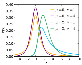
In probability theory, a log-t distribution or log-Student t distribution is a probability distribution of a random variable whose logarithm is distributed in accordance with a Student's t-distribution. If X is a random variable with a Student's t-distribution, then Y = exp(X) has a log-t distribution; likewise, if Y has a log-t distribution, then X = log(Y) has a Student's t-distribution.

References

↑ McKay, A. T. (1932). "Distribution of the coefficient of variation and the extended "t" distribution". Journal of the Royal Statistical Society. 95: 695–698. doi:10.2307/2342041.
↑ Iglevicz, Boris; Myers, Raymond (1970). "Comparisons of approximations to the percentage points of the sample coefficient of variation". Technometrics. 12 (1): 166–169. doi:10.2307/1267363. JSTOR 1267363.
↑ Bennett, B. M. (1976). "On an approximate test for homogeneity of coefficients of variation". Contributions to Applied Statistics Dedicated to A. Linder. Experentia Suppl. 22: 169–171.
↑ Vangel, Mark G. (1996). "Confidence intervals for a normal coefficient of variation". The American Statistician. 50 (1): 21–26. doi:10.1080/00031305.1996.10473537. JSTOR 2685039..
↑ Forkman, Johannes. "Estimator and tests for common coefficients of variation in normal distributions" (PDF). Communications in Statistics - Theory and Methods. pp. 21–26. doi:10.1080/03610920802187448 . Retrieved 2013-09-23.
↑ Forkman, Johannes; Verrill, Steve. "The distribution of McKay's approximation for the coefficient of variation" (PDF). Statistics & Probability Letters. pp. 10–14. doi:10.1016/j.spl.2007.04.018 . Retrieved 2013-09-23.

This page is based on this Wikipedia article
Text is available under the CC BY-SA 4.0 license; additional terms may apply.
Images, videos and audio are available under their respective licenses.

[1] McKay, A. T. (1932). "Distribution of the coefficient of variation and the extended "t" distribution". Journal of the Royal Statistical Society. 95: 695–698. doi:10.2307/2342041.

[2] Iglevicz, Boris; Myers, Raymond (1970). "Comparisons of approximations to the percentage points of the sample coefficient of variation". Technometrics. 12 (1): 166–169. doi:10.2307/1267363. JSTOR 1267363.

[3] Bennett, B. M. (1976). "On an approximate test for homogeneity of coefficients of variation". Contributions to Applied Statistics Dedicated to A. Linder. Experentia Suppl. 22: 169–171.

[4] Vangel, Mark G. (1996). "Confidence intervals for a normal coefficient of variation". The American Statistician. 50 (1): 21–26. doi:10.1080/00031305.1996.10473537. JSTOR 2685039..

[5] Forkman, Johannes. "Estimator and tests for common coefficients of variation in normal distributions" (PDF). Communications in Statistics - Theory and Methods. pp. 21–26. doi:10.1080/03610920802187448 . Retrieved 2013-09-23.

[6] Forkman, Johannes; Verrill, Steve. "The distribution of McKay's approximation for the coefficient of variation" (PDF). Statistics & Probability Letters. pp. 10–14. doi:10.1016/j.spl.2007.04.018 . Retrieved 2013-09-23.

[1]

[2]

[3]

[4]

[5]

[6]