The Phillips curve is an economic model, named after Bill Phillips, that correlates reduced unemployment with increasing wages in an economy. While Phillips did not directly link employment and inflation, this was a trivial deduction from his statistical findings. Paul Samuelson and Robert Solow made the connection explicit and subsequently Milton Friedman and Edmund Phelps put the theoretical structure in place.
In economics, the fiscal multiplier is the ratio of change in national income arising from a change in government spending. More generally, the exogenous spending multiplier is the ratio of change in national income arising from any autonomous change in spending. When this multiplier exceeds one, the enhanced effect on national income may be called the multiplier effect. The mechanism that can give rise to a multiplier effect is that an initial incremental amount of spending can lead to increased income and hence increased consumption spending, increasing income further and hence further increasing consumption, etc., resulting in an overall increase in national income greater than the initial incremental amount of spending. In other words, an initial change in aggregate demand may cause a change in aggregate output that is a multiple of the initial change.

In physics and fluid mechanics, a boundary layer is the thin layer of fluid in the immediate vicinity of a bounding surface formed by the fluid flowing along the surface. The fluid's interaction with the wall induces a no-slip boundary condition. The flow velocity then monotonically increases above the surface until it returns to the bulk flow velocity. The thin layer consisting of fluid whose velocity has not yet returned to the bulk flow velocity is called the velocity boundary layer.
In vector calculus, Green's theorem relates a line integral around a simple closed curve C to a double integral over the plane region D bounded by C. It is the two-dimensional special case of Stokes' theorem.
In economics, the marginal cost is the change in the total cost that arises when the quantity produced is increased, i.e. the cost of producing additional quantity. In some contexts, it refers to an increment of one unit of output, and in others it refers to the rate of change of total cost as output is increased by an infinitesimal amount. As Figure 1 shows, the marginal cost is measured in dollars per unit, whereas total cost is in dollars, and the marginal cost is the slope of the total cost, the rate at which it increases with output. Marginal cost is different from average cost, which is the total cost divided by the number of units produced.

In economics and in particular neoclassical economics, the marginal product or marginal physical productivity of an input is the change in output resulting from employing one more unit of a particular input, assuming that the quantities of other inputs are kept constant.
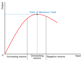
In economics, diminishing returns are the decrease in marginal (incremental) output of a production process as the amount of a single factor of production is incrementally increased, holding all other factors of production equal. The law of diminishing returns states that in productive processes, increasing a factor of production by one unit, while holding all other production factors constant, will at some point return a lower unit of output per incremental unit of input. The law of diminishing returns does not cause a decrease in overall production capabilities, rather it defines a point on a production curve whereby producing an additional unit of output will result in a loss and is known as negative returns. Under diminishing returns, output remains positive, but productivity and efficiency decrease.

Large eddy simulation (LES) is a mathematical model for turbulence used in computational fluid dynamics. It was initially proposed in 1963 by Joseph Smagorinsky to simulate atmospheric air currents, and first explored by Deardorff (1970). LES is currently applied in a wide variety of engineering applications, including combustion, acoustics, and simulations of the atmospheric boundary layer.
A time derivative is a derivative of a function with respect to time, usually interpreted as the rate of change of the value of the function. The variable denoting time is usually written as .
The Solow residual is a number describing empirical productivity growth in an economy from year to year and decade to decade. Robert Solow, the Nobel Memorial Prize in Economic Sciences-winning economist, defined rising productivity as rising output with constant capital and labor input. It is a "residual" because it is the part of growth that is not accounted for by measures of capital accumulation or increased labor input. Increased physical throughput – i.e. environmental resources – is specifically excluded from the calculation; thus some portion of the residual can be ascribed to increased physical throughput. The example used is for the intracapital substitution of aluminium fixtures for steel during which the inputs do not alter. This differs in almost every other economic circumstance in which there are many other variables. The Solow residual is procyclical and measures of it are now called the rate of growth of multifactor productivity or total factor productivity, though Solow (1957) did not use these terms.

A balanced budget is a budget in which revenues are equal to expenditures. Thus, neither a budget deficit nor a budget surplus exists. More generally, it is a budget that has no budget deficit, but could possibly have a budget surplus. A cyclically balanced budget is a budget that is not necessarily balanced year-to-year but is balanced over the economic cycle, running a surplus in boom years and running a deficit in lean years, with these offsetting over time.
The Solow–Swan model or exogenous growth model is an economic model of long-run economic growth. It attempts to explain long-run economic growth by looking at capital accumulation, labor or population growth, and increases in productivity largely driven by technological progress. At its core, it is an aggregate production function, often specified to be of Cobb–Douglas type, which enables the model "to make contact with microeconomics". The model was developed independently by Robert Solow and Trevor Swan in 1956, and superseded the Keynesian Harrod–Domar model.
The Harrod–Domar model is a Keynesian model of economic growth. It is used in development economics to explain an economy's growth rate in terms of the level of saving and of capital. It suggests that there is no natural reason for an economy to have balanced growth. The model was developed independently by Roy F. Harrod in 1939, and Evsey Domar in 1946, although a similar model had been proposed by Gustav Cassel in 1924. The Harrod–Domar model was the precursor to the exogenous growth model.

The GDP gap or the output gap is the difference between actual GDP or actual output and potential GDP, in an attempt to identify the current economic position over the business cycle. The measure of output gap is largely used in macroeconomic policy. The GDP gap is a highly criticized notion, in particular due to the fact that the potential GDP is not an observable variable, it is instead often derived from past GDP data, which could lead to systemic downward biases.
The Ramsey–Cass–Koopmans model, or Ramsey growth model, is a neoclassical model of economic growth based primarily on the work of Frank P. Ramsey, with significant extensions by David Cass and Tjalling Koopmans. The Ramsey–Cass–Koopmans model differs from the Solow–Swan model in that the choice of consumption is explicitly microfounded at a point in time and so endogenizes the savings rate. As a result, unlike in the Solow–Swan model, the saving rate may not be constant along the transition to the long run steady state. Another implication of the model is that the outcome is Pareto optimal or Pareto efficient.
The Incremental Capital-Output Ratio (ICOR) is the ratio of investment to growth which is equal to the reciprocal of the marginal product of capital. The higher the ICOR, the lower the productivity of capital or the marginal efficiency of capital. The ICOR can be thought of as a measure of the inefficiency with which capital is used. In most countries the ICOR is in the neighborhood of 3. It is a topic discussed in economic growth. It can be expressed in the following formula, where K is capital output ratio, Y is output (GDP), and I is net investment.
In fracture mechanics, the energy release rate, , is the rate at which energy is transformed as a material undergoes fracture. Mathematically, the energy release rate is expressed as the decrease in total potential energy per increase in fracture surface area, and is thus expressed in terms of energy per unit area. Various energy balances can be constructed relating the energy released during fracture to the energy of the resulting new surface, as well as other dissipative processes such as plasticity and heat generation. The energy release rate is central to the field of fracture mechanics when solving problems and estimating material properties related to fracture and fatigue.
In economics, the marginal product of labor (MPL) is the change in output that results from employing an added unit of labor. It is a feature of the production function and depends on the amounts of physical capital and labor already in use.
In monetary policy, the McCallum rule specifies a target for the monetary base (M0) which could be used by a central bank. The McCallum rule was proposed by Bennett T. McCallum at Carnegie Mellon University's Tepper School of Business. It is an alternative to the well known Taylor rule and performs better during crisis periods.
The AK model of economic growth is an endogenous growth model used in the theory of economic growth, a subfield of modern macroeconomics. In the 1980s it became progressively clearer that the standard neoclassical exogenous growth models were theoretically unsatisfactory as tools to explore long run growth, as these models predicted economies without technological change and thus they would eventually converge to a steady state, with zero per capita growth. A fundamental reason for this is the diminishing return of capital; the key property of AK endogenous-growth model is the absence of diminishing returns to capital. In lieu of the diminishing returns of capital implied by the usual parameterizations of a Cobb–Douglas production function, the AK model uses a linear model where output is a linear function of capital. Its appearance in most textbooks is to introduce endogenous growth theory.


