In mathematics, the Bernoulli numbersBn are a sequence of rational numbers which occur frequently in analysis. The Bernoulli numbers appear in the Taylor series expansions of the tangent and hyperbolic tangent functions, in Faulhaber's formula for the sum of m-th powers of the first n positive integers, in the Euler–Maclaurin formula, and in expressions for certain values of the Riemann zeta function.

In mathematics, the Taylor series or Taylor expansion of a function is an infinite sum of terms that are expressed in terms of the function's derivatives at a single point. For most common functions, the function and the sum of its Taylor series are equal near this point. Taylor series are named after Brook Taylor, who introduced them in 1715. A Taylor series is also called a Maclaurin series when 0 is the point where the derivatives are considered, after Colin Maclaurin, who made extensive use of this special case of Taylor series in the 18th century.

In numerical analysis, an n-point Gaussian quadrature rule, named after Carl Friedrich Gauss, is a quadrature rule constructed to yield an exact result for polynomials of degree 2n − 1 or less by a suitable choice of the nodes xi and weights wi for i = 1, ..., n.

In calculus, Taylor's theorem gives an approximation of a -times differentiable function around a given point by a polynomial of degree , called the -th-order Taylor polynomial. For a smooth function, the Taylor polynomial is the truncation at the order of the Taylor series of the function. The first-order Taylor polynomial is the linear approximation of the function, and the second-order Taylor polynomial is often referred to as the quadratic approximation. There are several versions of Taylor's theorem, some giving explicit estimates of the approximation error of the function by its Taylor polynomial.

In analysis, numerical integration comprises a broad family of algorithms for calculating the numerical value of a definite integral. The term numerical quadrature is more or less a synonym for "numerical integration", especially as applied to one-dimensional integrals. Some authors refer to numerical integration over more than one dimension as cubature; others take "quadrature" to include higher-dimensional integration.

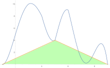
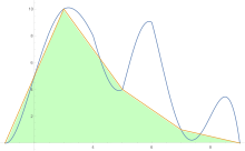
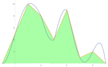
In numerical analysis, the Lagrange interpolating polynomial is the unique polynomial of lowest degree that interpolates a given set of data.

In statistics, Spearman's rank correlation coefficient or Spearman's ρ, named after Charles Spearman and often denoted by the Greek letter (rho) or as , is a nonparametric measure of rank correlation. It assesses how well the relationship between two variables can be described using a monotonic function.
In finance, the rule of 72, the rule of 70 and the rule of 69.3 are methods for estimating an investment's doubling time. The rule number is divided by the interest percentage per period to obtain the approximate number of periods required for doubling. Although scientific calculators and spreadsheet programs have functions to find the accurate doubling time, the rules are useful for mental calculations and when only a basic calculator is available.

In numerical analysis, Richardson extrapolation is a sequence acceleration method used to improve the rate of convergence of a sequence of estimates of some value . In essence, given the value of for several values of , we can estimate by extrapolating the estimates to . It is named after Lewis Fry Richardson, who introduced the technique in the early 20th century, though the idea was already known to Christiaan Huygens in his calculation of . In the words of Birkhoff and Rota, "its usefulness for practical computations can hardly be overestimated."
In statistics, G-tests are likelihood-ratio or maximum likelihood statistical significance tests that are increasingly being used in situations where chi-squared tests were previously recommended.

The rectangular function is defined as

In mathematics and computational science, the Euler method is a first-order numerical procedure for solving ordinary differential equations (ODEs) with a given initial value. It is the most basic explicit method for numerical integration of ordinary differential equations and is the simplest Runge–Kutta method. The Euler method is named after Leonhard Euler, who first proposed it in his book Institutionum calculi integralis.
Adaptive Simpson's method, also called adaptive Simpson's rule, is a method of numerical integration proposed by G.F. Kuncir in 1962. It is probably the first recursive adaptive algorithm for numerical integration to appear in print, although more modern adaptive methods based on Gauss–Kronrod quadrature and Clenshaw–Curtis quadrature are now generally preferred. Adaptive Simpson's method uses an estimate of the error we get from calculating a definite integral using Simpson's rule. If the error exceeds a user-specified tolerance, the algorithm calls for subdividing the interval of integration in two and applying adaptive Simpson's method to each subinterval in a recursive manner. The technique is usually much more efficient than composite Simpson's rule since it uses fewer function evaluations in places where the function is well-approximated by a cubic function.
In numerical analysis and linear algebra, lower–upper (LU) decomposition or factorization factors a matrix as the product of a lower triangular matrix and an upper triangular matrix. The product sometimes includes a permutation matrix as well. LU decomposition can be viewed as the matrix form of Gaussian elimination. Computers usually solve square systems of linear equations using LU decomposition, and it is also a key step when inverting a matrix or computing the determinant of a matrix. The LU decomposition was introduced by the Polish astronomer Tadeusz Banachiewicz in 1938. To quote: "It appears that Gauss and Doolittle applied the method [of elimination] only to symmetric equations. More recent authors, for example, Aitken, Banachiewicz, Dwyer, and Crout … have emphasized the use of the method, or variations of it, in connection with non-symmetric problems … Banachiewicz … saw the point … that the basic problem is really one of matrix factorization, or “decomposition” as he called it." It is also sometimes referred to as LR decomposition.
In statistics, the Kendall rank correlation coefficient, commonly referred to as Kendall's τ coefficient, is a statistic used to measure the ordinal association between two measured quantities. A τ test is a non-parametric hypothesis test for statistical dependence based on the τ coefficient. It is a measure of rank correlation: the similarity of the orderings of the data when ranked by each of the quantities. It is named after Maurice Kendall, who developed it in 1938, though Gustav Fechner had proposed a similar measure in the context of time series in 1897.
Stochastic approximation methods are a family of iterative methods typically used for root-finding problems or for optimization problems. The recursive update rules of stochastic approximation methods can be used, among other things, for solving linear systems when the collected data is corrupted by noise, or for approximating extreme values of functions which cannot be computed directly, but only estimated via noisy observations.

In mathematical analysis, the Dirichlet kernel, named after the German mathematician Peter Gustav Lejeune Dirichlet, is the collection of periodic functions defined as

In mathematics, Ramanujan's Master Theorem, named after Srinivasa Ramanujan, is a technique that provides an analytic expression for the Mellin transform of an analytic function.
The spectral correlation density (SCD), sometimes also called the cyclic spectral density or spectral correlation function, is a function that describes the cross-spectral density of all pairs of frequency-shifted versions of a time-series. The spectral correlation density applies only to cyclostationary processes because stationary processes do not exhibit spectral correlation. Spectral correlation has been used both in signal detection and signal classification. The spectral correlation density is closely related to each of the bilinear time-frequency distributions, but is not considered one of Cohen's class of distributions.