The state-transition equation is defined as the solution of the linear homogeneous state equation. The linear time-invariant state equation given by
with state vector x, control vector u, vector w of additive disturbances, and fixed matrices A, B, and E, can be solved by using either the classical method of solving linear differential equations or the Laplace transform method. The Laplace transform solution is presented in the following equations. The Laplace transform of the above equation yields
where x(0) denotes initial-state vector evaluated at . Solving for gives
So, the state-transition equation can be obtained by taking inverse Laplace transform as
The state-transition equation as derived above is useful only when the initial time is defined to be at . In the study of control systems, specially discrete-data control systems, it is often desirable to break up a state-transition process into a sequence of transitions, so a more flexible initial time must be chosen. Let the initial time be represented by and the corresponding initial state by , and assume that the input and the disturbance are applied at t≥0. Starting with the above equation by setting and solving for , we get
Once the state-transition equation is determined, the output vector can be expressed as a function of the initial state.
The step response of a system in a given initial state consists of the time evolution of its outputs when its control inputs are Heaviside step functions. In electronic engineering and control theory, step response is the time behaviour of the outputs of a general system when its inputs change from zero to one in a very short time. The concept can be extended to the abstract mathematical notion of a dynamical system using an evolution parameter.
In physics, the S-matrix or scattering matrix relates the initial state and the final state of a physical system undergoing a scattering process. It is used in quantum mechanics, scattering theory and quantum field theory (QFT).
The adiabatic theorem is a concept in quantum mechanics. Its original form, due to Max Born and Vladimir Fock (1928), was stated as follows:
In physics, the Hamilton–Jacobi equation, named after William Rowan Hamilton and Carl Gustav Jacob Jacobi, is an alternative formulation of classical mechanics, equivalent to other formulations such as Newton's laws of motion, Lagrangian mechanics and Hamiltonian mechanics.
In system analysis, among other fields of study, a linear time-invariant (LTI) system is a system that produces an output signal from any input signal subject to the constraints of linearity and time-invariance; these terms are briefly defined below. These properties apply (exactly or approximately) to many important physical systems, in which case the response y(t) of the system to an arbitrary input x(t) can be found directly using convolution: y(t) = (x ∗ h)(t) where h(t) is called the system's impulse response and ∗ represents convolution (not to be confused with multiplication). What's more, there are systematic methods for solving any such system (determining h(t)), whereas systems not meeting both properties are generally more difficult (or impossible) to solve analytically. A good example of an LTI system is any electrical circuit consisting of resistors, capacitors, inductors and linear amplifiers.
In mathematics, the discrete Laplace operator is an analog of the continuous Laplace operator, defined so that it has meaning on a graph or a discrete grid. For the case of a finite-dimensional graph, the discrete Laplace operator is more commonly called the Laplacian matrix.
In algebra, the Bring radical or ultraradical of a real number a is the unique real root of the polynomial
In control theory, a distributed-parameter system is a system whose state space is infinite-dimensional. Such systems are therefore also known as infinite-dimensional systems. Typical examples are systems described by partial differential equations or by delay differential equations.
In mathematics, delay differential equations (DDEs) are a type of differential equation in which the derivative of the unknown function at a certain time is given in terms of the values of the function at previous times. DDEs are also called time-delay systems, systems with aftereffect or dead-time, hereditary systems, equations with deviating argument, or differential-difference equations. They belong to the class of systems with the functional state, i.e. partial differential equations (PDEs) which are infinite dimensional, as opposed to ordinary differential equations (ODEs) having a finite dimensional state vector. Four points may give a possible explanation of the popularity of DDEs:
Aftereffect is an applied problem: it is well known that, together with the increasing expectations of dynamic performances, engineers need their models to behave more like the real process. Many processes include aftereffect phenomena in their inner dynamics. In addition, actuators, sensors, and communication networks that are now involved in feedback control loops introduce such delays. Finally, besides actual delays, time lags are frequently used to simplify very high order models. Then, the interest for DDEs keeps on growing in all scientific areas and, especially, in control engineering.
Delay systems are still resistant to many classical controllers: one could think that the simplest approach would consist in replacing them by some finite-dimensional approximations. Unfortunately, ignoring effects which are adequately represented by DDEs is not a general alternative: in the best situation, it leads to the same degree of complexity in the control design. In worst cases, it is potentially disastrous in terms of stability and oscillations.
Voluntary introduction of delays can benefit the control system.
In spite of their complexity, DDEs often appear as simple infinite-dimensional models in the very complex area of partial differential equations (PDEs).
Toroidal coordinates are a three-dimensional orthogonal coordinate system that results from rotating the two-dimensional bipolar coordinate system about the axis that separates its two foci. Thus, the two foci and in bipolar coordinates become a ring of radius in the plane of the toroidal coordinate system; the -axis is the axis of rotation. The focal ring is also known as the reference circle.
Oblate spheroidal coordinates are a three-dimensional orthogonal coordinate system that results from rotating the two-dimensional elliptic coordinate system about the non-focal axis of the ellipse, i.e., the symmetry axis that separates the foci. Thus, the two foci are transformed into a ring of radius in the x-y plane. Oblate spheroidal coordinates can also be considered as a limiting case of ellipsoidal coordinates in which the two largest semi-axes are equal in length.
In control theory, we may need to find out whether or not a system such as
The theoretical and experimental justification for the Schrödinger equation motivates the discovery of the Schrödinger equation, the equation that describes the dynamics of nonrelativistic particles. The motivation uses photons, which are relativistic particles with dynamics described by Maxwell's equations, as an analogue for all types of particles.
Sediment transport is the movement of solid particles (sediment), typically due to a combination of gravity acting on the sediment, and the movement of the fluid in which the sediment is entrained. Sediment transport occurs in natural systems where the particles are clastic rocks, mud, or clay; the fluid is air, water, or ice; and the force of gravity acts to move the particles along the sloping surface on which they are resting. Sediment transport due to fluid motion occurs in rivers, oceans, lakes, seas, and other bodies of water due to currents and tides. Transport is also caused by glaciers as they flow, and on terrestrial surfaces under the influence of wind. Sediment transport due only to gravity can occur on sloping surfaces in general, including hillslopes, scarps, cliffs, and the continental shelf—continental slope boundary.
The geodetic effect represents the effect of the curvature of spacetime, predicted by general relativity, on a vector carried along with an orbiting body. For example, the vector could be the angular momentum of a gyroscope orbiting the Earth, as carried out by the Gravity Probe B experiment. The geodetic effect was first predicted by Willem de Sitter in 1916, who provided relativistic corrections to the Earth–Moon system's motion. De Sitter's work was extended in 1918 by Jan Schouten and in 1920 by Adriaan Fokker. It can also be applied to a particular secular precession of astronomical orbits, equivalent to the rotation of the Laplace–Runge–Lenz vector.
The intent of this article is to highlight the important points of the derivation of the Navier–Stokes equations as well as its application and formulation for different families of fluids.
The Cauchy momentum equation is a vector partial differential equation put forth by Cauchy that describes the non-relativistic momentum transport in any continuum.
In control theory, the state-transition matrix is a matrix whose product with the state vector at an initial time gives at a later time . The state-transition matrix can be used to obtain the general solution of linear dynamical systems.
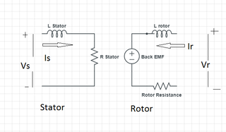
An armature controlled DC motor is a direct current (DC) motor that uses a permanent magnet driven by the armature coils only.
The Cole–Hopf transformation is a method of solving parabolic partial differential equations (PDEs) with a quadratic nonlinearity of the form:
This page is based on this Wikipedia article Text is available under the CC BY-SA 4.0 license; additional terms may apply. Images, videos and audio are available under their respective licenses.