Bresenham's line algorithm

Bresenham's line algorithm is a line drawing algorithm that determines the points of an n-dimensional raster that should be selected in order to form a close approximation to a straight line between two points. It is commonly used to draw line primitives in a bitmap image (e.g. on a computer screen), as it uses only integer addition, subtraction, and bit shifting, all of which are very cheap operations in historically common computer architectures. It is an incremental error algorithm, and one of the earliest algorithms developed in the field of computer graphics. An extension to the original algorithm called the midpoint circle algorithm may be used for drawing circles.

While algorithms such as Wu's algorithm are also frequently used in modern computer graphics because they can support antialiasing, Bresenham's line algorithm is still important because of its speed and simplicity. The algorithm is used in hardware such as plotters and in the graphics chips of modern graphics cards. It can also be found in many software graphics libraries. Because the algorithm is very simple, it is often implemented in either the firmware or the graphics hardware of modern graphics cards.

The label "Bresenham" is used today for a family of algorithms extending or modifying Bresenham's original algorithm.

History

Bresenham's line algorithm is named after Jack Elton Bresenham who developed it in 1962 at IBM. In 2001 Bresenham wrote: ^[1]

I was working in the computation lab at IBM's San Jose development lab. A Calcomp plotter had been attached to an IBM 1401 via the 1407 typewriter console. [The algorithm] was in production use by summer 1962, possibly a month or so earlier. Programs in those days were freely exchanged among corporations so Calcomp (Jim Newland and Calvin Hefte) had copies. When I returned to Stanford in Fall 1962, I put a copy in the Stanford comp center library. A description of the line drawing routine was accepted for presentation at the 1963 ACM national convention in Denver, Colorado. It was a year in which no proceedings were published, only the agenda of speakers and topics in an issue of Communications of the ACM. A person from the IBM Systems Journal asked me after I made my presentation if they could publish the paper. I happily agreed, and they printed it in 1965.

Method

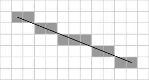
Illustration of the result of Bresenham's line algorithm. (0,0) is at the top left corner of the grid, (1,1) is at the top left end of the line and (11, 5) is at the bottom right end of the line.

The following conventions will be utilized:

• the top-left is (0,0) such that pixel coordinates increase in the right and down directions (e.g. that the pixel at (7,4) is directly above the pixel at (7,5)), and
• the pixel centers have integer coordinates.

The endpoints of the line are the pixels at ${\displaystyle (x_{0},y_{0})}$ and ${\displaystyle (x_{1},y_{1})}$, where the first coordinate of the pair is the column and the second is the row.

The algorithm will be initially presented only for the octant in which the segment goes down and to the right (${\displaystyle x_{0}\leq x_{1}}$ and ${\displaystyle y_{0}\leq y_{1}}$), and its horizontal projection ${\displaystyle x_{1}-x_{0}}$ is longer than the vertical projection ${\displaystyle y_{1}-y_{0}}$ (the line has a positive slope less than 1). In this octant, for each column x between ${\displaystyle x_{0}}$ and ${\displaystyle x_{1}}$, there is exactly one row y (computed by the algorithm) containing a pixel of the line, while each row between ${\displaystyle y_{0}}$ and ${\displaystyle y_{1}}$ may contain multiple rasterized pixels.

Bresenham's algorithm chooses the integer y corresponding to the pixel center that is closest to the ideal (fractional) y for the same x; on successive columns y can remain the same or increase by 1. The general equation of the line through the endpoints is given by:

${\displaystyle {\frac {y-y_{0}}{y_{1}-y_{0}}}={\frac {x-x_{0}}{x_{1}-x_{0}}}}$.

Since we know the column, x, the pixel's row, y, is given by rounding this quantity to the nearest integer:

${\displaystyle y={\frac {y_{1}-y_{0}}{x_{1}-x_{0}}}(x-x_{0})+y_{0}}$.

The slope ${\displaystyle (y_{1}-y_{0})/(x_{1}-x_{0})}$ depends on the endpoint coordinates only and can be precomputed, and the ideal y for successive integer values of x can be computed starting from ${\displaystyle y_{0}}$ and repeatedly adding the slope.

In practice, the algorithm does not keep track of the y coordinate, which increases by m = ∆y/∆x each time the x increases by one; it keeps an error bound at each stage, which represents the negative of the distance from (a) the point where the line exits the pixel to (b) the top edge of the pixel. This value is first set to ${\displaystyle y_{0}-0.5}$ (due to using the pixel's center coordinates), and is incremented by m each time the x coordinate is incremented by one. If the error becomes greater than 0.5, we know that the line has moved upwards one pixel, and that we must increment our y coordinate and readjust the error to represent the distance from the top of the new pixel – which is done by subtracting one from error. ^[2]

Derivation

To derive Bresenham's algorithm, two steps must be taken. The first step is transforming the equation of a line from the typical slope-intercept form into something different; and then using this new equation to draw a line based on the idea of accumulation of error.

Line equation

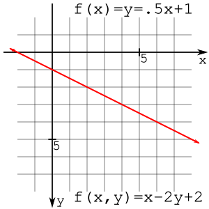
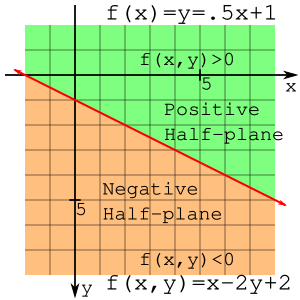
y=f(x)=.5x+1 or f(x,y)=x-2y+2=0

Positive and negative half-planes

The slope-intercept form of a line is written as

${\displaystyle y=f(x)=mx+b}$

where ${\displaystyle m}$ is the slope and ${\displaystyle b}$ is the y-intercept. Because this is a function of only ${\displaystyle x}$, it can't represent a vertical line. Therefore, it would be useful to make this equation written as a function of both ${\displaystyle x}$and${\displaystyle y}$, to be able to draw lines at any angle. The angle (or slope) of a line can be stated as "rise over run", or ${\displaystyle \Delta y/\Delta x}$. Then, using algebraic manipulation,

${\displaystyle {\begin{aligned}y&=mx+b\\y&={\frac {\Delta y}{\Delta x}}x+b\\(\Delta x)y&=(\Delta y)x+(\Delta x)b\\0&=(\Delta y)x-(\Delta x)y+(\Delta x)b\end{aligned}}}$

Letting this last equation be a function of ${\displaystyle x}$ and ${\displaystyle y}$, it can be written as

${\displaystyle f(x,y):=Ax+By+C=0}$

where the constants are

• ${\displaystyle A=\Delta y=y_{1}-y_{0}}$
• ${\displaystyle B=-\Delta x=-(x_{1}-x_{0})}$
• ${\displaystyle C=(\Delta x)b=(x_{1}-x_{0})b}$

The line is then defined for some constants ${\displaystyle A}$, ${\displaystyle B}$, and ${\displaystyle C}$ anywhere ${\displaystyle f(x,y)=0}$. That is, for any ${\displaystyle (x,y)}$ not on the line, ${\displaystyle f(x,y)\neq 0}$. This form involves only integers if ${\displaystyle x}$ and ${\displaystyle y}$ are integers, since the constants ${\displaystyle A}$, ${\displaystyle B}$, and ${\displaystyle C}$ are defined as integers.

As an example, the line ${\textstyle y={\frac {1}{2}}x+1}$ then this could be written as ${\displaystyle f(x,y)=x-2y+2}$. The point (2,2) is on the line

${\displaystyle f(2,2)=x-2y+2=(2)-2(2)+2=2-4+2=0}$

and the point (2,3) is not on the line

${\displaystyle f(2,3)=(2)-2(3)+2=2-6+2=-2}$

and neither is the point (2,1)

${\displaystyle f(2,1)=(2)-2(1)+2=2-2+2=2}$

Notice that the points (2,1) and (2,3) are on opposite sides of the line and ${\displaystyle f(x,y)}$ evaluates to positive or negative. A line splits a plane into halves and the half-plane that has a negative ${\displaystyle f(x,y)}$ can be called the negative half-plane, and the other half can be called the positive half-plane. This observation is very important in the remainder of the derivation.

Algorithm

Clearly, the starting point is on the line

${\displaystyle f(x_{0},y_{0})=0}$

only because the line is defined to start and end on integer coordinates (though it is entirely reasonable to want to draw a line with non-integer end points).

Candidate point (2,2) in blue and two candidate points in green (3,2) and (3,3)

Keeping in mind that the slope is at most ${\displaystyle 1}$, the problem now presents itself as to whether the next point should be at ${\displaystyle (x_{0}+1,y_{0})}$ or ${\displaystyle (x_{0}+1,y_{0}+1)}$. Perhaps intuitively, the point should be chosen based upon which is closer to the line at ${\displaystyle x_{0}+1}$. If it is closer to the former then include the former point on the line, if the latter then the latter. To answer this, evaluate the line function at the midpoint between these two points:

${\displaystyle f(x_{0}+1,y_{0}+{\tfrac {1}{2}})}$

If the value of this is positive then the ideal line is below the midpoint and closer to the candidate point ${\displaystyle (x_{0}+1,y_{0}+1)}$; i.e. the y coordinate should increase. Otherwise, the ideal line passes through or above the midpoint, and the y coordinate should stay the same; in which case the point ${\displaystyle (x_{0}+1,y_{0})}$ is chosen. The value of the line function at this midpoint is the sole determinant of which point should be chosen.

The adjacent image shows the blue point (2,2) chosen to be on the line with two candidate points in green (3,2) and (3,3). The black point (3, 2.5) is the midpoint between the two candidate points.

Algorithm for integer arithmetic

Alternatively, the difference between points can be used instead of evaluating f(x,y) at midpoints. This alternative method allows for integer-only arithmetic, which is generally faster than using floating-point arithmetic. To derive the other method, define the difference to be as follows:

${\displaystyle D=f(x_{0}+1,y_{0}+{\tfrac {1}{2}})-f(x_{0},y_{0})}$

For the first decision, this formulation is equivalent to the midpoint method since ${\displaystyle f(x_{0},y_{0})=0}$ at the starting point. Simplifying this expression yields:

${\displaystyle {\begin{array}{rclcl}D&=&\left[A(x_{0}+1)+B\left(y_{0}+{\frac {1}{2}}\right)+C\right]&-&\left[Ax_{0}+By_{0}+C\right]\\&=&\left[Ax_{0}+By_{0}+C+A+{\frac {1}{2}}B\right]&-&\left[Ax_{0}+By_{0}+C\right]\\&=&A+{\frac {1}{2}}B=\Delta y-{\frac {1}{2}}\Delta x\end{array}}}$

Just as with the midpoint method, if ${\displaystyle D}$ is positive, then choose ${\displaystyle (x_{0}+1,y_{0}+1)}$, otherwise choose ${\displaystyle (x_{0}+1,y_{0})}$.

If ${\displaystyle (x_{0}+1,y_{0})}$ is chosen, the change in D will be:

${\displaystyle {\begin{array}{lclcl}\Delta D&=&f(x_{0}+2,y_{0}+{\tfrac {1}{2}})-f(x_{0}+1,y_{0}+{\tfrac {1}{2}})&=&A&=&\Delta y\\\end{array}}}$

If ${\displaystyle (x_{0}+1,y_{0}+1)}$ is chosen the change in D will be:

${\displaystyle {\begin{array}{lclcl}\Delta D&=&f(x_{0}+2,y_{0}+{\tfrac {3}{2}})-f(x_{0}+1,y_{0}+{\tfrac {1}{2}})&=&A+B&=&\Delta y-\Delta x\end{array}}}$

If the new D is positive then ${\displaystyle (x_{0}+2,y_{0}+1)}$ is chosen, otherwise ${\displaystyle (x_{0}+2,y_{0})}$. This decision can be generalized by accumulating the error on each subsequent point.

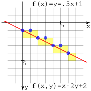
Plotting the line from (0,1) to (6,4) showing a plot of grid lines and pixels

All of the derivation for the algorithm is done. One performance issue is the 1/2 factor in the initial value of D. Since all of this is about the sign of the accumulated difference, then everything can be multiplied by 2 with no consequence.

This results in an algorithm that uses only integer arithmetic.

plotLine(x0, y0, x1, y1)     dx = x1 - x0     dy = y1 - y0     D = 2*dy - dx     y = y0      for x from x0 to x1         plot(x, y)         if D > 0             y = y + 1             D = D - 2*dx         end if         D = D + 2*dy

Running this algorithm for ${\displaystyle f(x,y)=x-2y+2}$ from (0,1) to (6,4) yields the following differences with dx=6 and dy=3:

D=2*3-6=0 Loop from 0 to 6  * x=0: plot(0, 1), D≤0: D=0+6=6  * x=1: plot(1, 1), D>0: D=6-12=-6, y=1+1=2, D=-6+6=0  * x=2: plot(2, 2), D≤0: D=0+6=6  * x=3: plot(3, 2), D>0: D=6-12=-6, y=2+1=3, D=-6+6=0  * x=4: plot(4, 3), D≤0: D=0+6=6  * x=5: plot(5, 3), D>0: D=6-12=-6, y=3+1=4, D=-6+6=0  * x=6: plot(6, 4), D≤0: D=0+6=6

The result of this plot is shown to the right. The plotting can be viewed by plotting at the intersection of lines (blue circles) or filling in pixel boxes (yellow squares). Regardless, the plotting is the same.

All cases

However, as mentioned above this only works for octant zero, that is lines starting at the origin with a slope between 0 and 1 where x increases by exactly 1 per iteration and y increases by 0 or 1.

The algorithm can be extended to cover slopes between 0 and -1 by checking whether y needs to increase or decrease (i.e. dy < 0)

plotLineLow(x0, y0, x1, y1)     dx = x1 - x0     dy = y1 - y0     yi = 1     if dy < 0         yi = -1         dy = -dy     end if     D = (2 * dy) - dx     y = y0      for x from x0 to x1         plot(x, y)         if D > 0             y = y + yi             D = D + (2 * (dy - dx))         else             D = D + 2*dy         end if

By switching the x and y axis an implementation for positive or negative steep slopes can be written as

plotLineHigh(x0, y0, x1, y1)     dx = x1 - x0     dy = y1 - y0     xi = 1     if dx < 0         xi = -1         dx = -dx     end if     D = (2 * dx) - dy     x = x0      for y from y0 to y1         plot(x, y)         if D > 0             x = x + xi             D = D + (2 * (dx - dy))         else             D = D + 2*dx         end if

A complete solution would need to detect whether x1 > x0 or y1 > y0 and reverse the input coordinates before drawing, thus

plotLine(x0, y0, x1, y1)     if abs(y1 - y0) < abs(x1 - x0)         if x0 > x1             plotLineLow(x1, y1, x0, y0)         else             plotLineLow(x0, y0, x1, y1)         end ifelseif y0 > y1             plotLineHigh(x1, y1, x0, y0)         else             plotLineHigh(x0, y0, x1, y1)         end ifend if

In low level implementations which access the video memory directly, it would be typical for the special cases of vertical and horizontal lines to be handled separately as they can be highly optimized.

Some versions use Bresenham's principles of integer incremental error to perform all octant line draws, balancing the positive and negative error between the x and y coordinates. ^[3]

plotLine(x0, y0, x1, y1)     dx = abs(x1 - x0)     sx = x0 < x1 ? 1 : -1     dy = -abs(y1 - y0)     sy = y0 < y1 ? 1 : -1     error = dx + dy          while true         plot(x0, y0)         if x0 == x1 && y0 == y1 break         e2 = 2 * error         if e2 >= dy             if x0 == x1 break             error = error + dy             x0 = x0 + sx         end ifif e2 <= dx             if y0 == y1 break             error = error + dx             y0 = y0 + sy         end ifend while

Similar algorithms

The Bresenham algorithm can be interpreted as slightly modified digital differential analyzer (using 0.5 as error threshold instead of 0, which is required for non-overlapping polygon rasterizing).

The principle of using an incremental error in place of division operations has other applications in graphics. It is possible to use this technique to calculate the U,V co-ordinates during raster scan of texture mapped polygons. ^[4] The voxel heightmap software-rendering engines seen in some PC games also used this principle.

Bresenham also published a Run-Slice computational algorithm: while the above described Run-Length algorithm runs the loop on the major axis, the Run-Slice variation loops the other way. ^[5] This method has been represented in a number of US patents:

5,815,163		Method and apparatus to draw line slices during calculation
5,740,345		Method and apparatus for displaying computer graphics data stored in a compressed format with an efficient color indexing system
5,657,435		Run slice line draw engine with non-linear scaling capabilities
5,627,957		Run slice line draw engine with enhanced processing capabilities
5,627,956		Run slice line draw engine with stretching capabilities
5,617,524		Run slice line draw engine with shading capabilities
5,611,029		Run slice line draw engine with non-linear shading capabilities
5,604,852		Method and apparatus for displaying a parametric curve on a video display
5,600,769		Run slice line draw engine with enhanced clipping techniques

The algorithm has been extended to:

• Draw lines of arbitrary thickness, an algorithm created by Alan Murphy at IBM. ^[6]
• Draw multiple kinds curves (circles, ellipses, cubic, quadratic, and rational bezier curves) and antialiased lines and curves; a set of algorithms by Alois Zingl. ^[3]

See also

• Digital differential analyzer (graphics algorithm), a simple and general method for rasterizing lines and triangles
• Xiaolin Wu's line algorithm, a similarly fast method of drawing lines with antialiasing
• Midpoint circle algorithm, a similar algorithm for drawing circles

Notes

1. Paul E. Black. Dictionary of Algorithms and Data Structures, NIST. https://xlinux.nist.gov/dads/HTML/bresenham.html
2. Joy, Kenneth. "Bresenham's Algorithm" (PDF). Visualization and Graphics Research Group, Department of Computer Science, University of California, Davis. Retrieved 20 December 2016.
3. Zingl, Alois (2012). A Rasterizing Algorithm for Drawing Curves (PDF) (Report).
   HTML abstract and demo: Zingl, Alois (2016). "Bresenham". members.chello.at.
4. US 5739818,Spackman, John Neil,"Apparatus and method for performing perspectively correct interpolation in computer graphics",published 1998-04-14, assigned to Canon KK  
5. "Michael Abrash's Graphics Programming Black Book Special Edition: The Good, the Bad, and the Run-Sliced". www.phatcode.net. Retrieved 13 February 2024.;
6. "Murphy's Modified Bresenham Line Algorithm". homepages.enterprise.net. Retrieved 2018-06-09. ('Line Thickening by Modification to Bresenham's Algorithm' in the IBM Technical Disclosure Bulletin Vol. 20 No. 12 May 1978 pages 5358-5366.)

References

• Bresenham, J. E. (1965). "Algorithm for computer control of a digital plotter" (PDF). IBM Systems Journal. 4 (1): 25–30. doi:10.1147/sj.41.0025. Archived from the original (PDF) on May 28, 2008.
• "The Bresenham Line-Drawing Algorithm", by Colin Flanagan
• Abrash, Michael (1997). Michael Abrash's graphics programming black book . Albany, NY: Coriolis. pp.  654–678. ISBN   978-1-57610-174-2. A very optimized version of the algorithm in C and assembly for use in video games with complete details of its inner workings
• Zingl, Alois (2012). "A Rasterizing Algorithm for Drawing Curves" (PDF)., The Beauty of Bresenham's Algorithms

Further reading

• Patrick-Gillesbanda Thesis, containing an extension of the Bresenham line drawing algorithm to perform 3D hidden lines removal
  • also published in MICAD '87 proceedings on CAD/CAM and Computer Graphics, page 591 - ISBN   2-86601-084-1.
• Line Thickening by Modification To Bresenham's Algorithm, A.S. Murphy, IBM Technical Disclosure Bulletin, Vol. 20, No. 12, May 1978.
• Bresenham, Jack (February 1977). "A linear algorithm for incremental digital display of circular arcs". Communications of the ACM. 20 (2): 100–106. doi:10.1145/359423.359432.– also Technical Report 1964 Jan-27 -11- Circle Algorithm TR-02-286 IBM San Jose Lab

External links

• Michael Abrash's Graphics Programming Black Book Special Edition: Chapter 35: Bresenham Is Fast, and Fast Is Good
• The Bresenham Line-Drawing Algorithm by Colin Flanagan
• National Institute of Standards and Technology page on Bresenham's algorithm
• Calcomp 563 Incremental Plotter Information
• Bresenham Algorithm in several programming languages
• The Beauty of Bresenham's Algorithm – A simple implementation to plot lines, circles, ellipses and Bézier curves