Chromatographic response function

Last updated April 12, 2024

Chromatographic response function, often abbreviated to CRF, is a coefficient which measures the quality of the separation in the result of a chromatography.

Examples in thin layer chromatography

The CRFs in thin layer chromatography characterize the equal-spreading of the spots. The ideal case, when the RF of the spots are uniformly distributed in <0,1> range (for example 0.25,0.5 and 0.75 for three solutes) should be characterized as the best situation possible.

The simplest criteria are $\Delta R_{F}$ and $\Delta R_{F}$ product (Wang et al., 1996). They are the smallest difference between sorted RF values, or product of such differences.

Another function is the multispot response function (MRF) as developed by De Spiegeleer et al.{Analytical Chemistry (1987):59(1),62-64} It is based also of differences product. This function always lies between 0 and 1. When two RF values are equal, it is equal to 0, when all RF values are equal-spread, it is equal to 1. The L and U values – upper and lower limit of RF – give possibility to avoid the band region.

$MRF={\frac {(U-hR_{Fn})(hR_{F1}-L)\prod _{i=1}^{n-1}(hR_{Fi+1}-hR_{Fi})}{[(U-L)/(n+1)]^{n+1}}}$

The last example of coefficient sensitive to minimal distance between spots is Retention distance (Komsta et al., 2007)

$R_{D}={\Bigg [}(n+1)^{(n+1)}\prod _{i=0}^{n}{(R_{F(i+1)}-R_{Fi}){\Bigg ]}^{\frac {1}{n}}}$

The second group are criteria insensitive for minimal difference between RF values (if two compounds are not separated, such CRF functions will not indicate it). They are equal to zero in equal-spread state increase when situation is getting worse.

There are:

Separation response (Bayne et al., 1987)

$D={\sqrt {\sum _{i=1}^{n}\left(R_{Fi}-{\frac {i-1}{n-1}}\right)}}$

Performance index (Gocan et al., 1991)

$I_{p}={\sqrt {\frac {\sum (\Delta hR_{Fi}-\Delta hR_{Ft})^{2}}{n(n+1)}}}$

Informational entropy (Gocan et al., 1991, second reference)

$s_{m}={\sqrt {\frac {\sum (\Delta hR_{Fi}-\Delta hR_{Ft})^{2}}{n+1}}}$

Retention uniformity (Komsta et al., 2007)

$R_{U}=1-{\sqrt {{\frac {6(n+1)}{n(2n+1)}}\sum _{i=1}^{n}{\left(R_{Fi}-{\frac {i}{n+1}}\right)^{2}}}}$

In all above formulas, n is the number of compounds separated, R_{f (1...n)} are the Retention factor of the compounds sorted in non-descending order, R_f0 = 0 and R_f(n+1) = 1.

Related Research Articles

In probability theory and statistics, kurtosis is a measure of the "tailedness" of the probability distribution of a real-valued random variable. Like skewness, kurtosis describes a particular aspect of a probability distribution. There are different ways to quantify kurtosis for a theoretical distribution, and there are corresponding ways of estimating it using a sample from a population. Different measures of kurtosis may have different interpretations.

The natural logarithm of a number is its logarithm to the base of the mathematical constant $e$ , which is an irrational and transcendental number approximately equal to $2.718 281828459$ . The natural logarithm of $x$ is generally written as $ln x$ , $log e x$ , or sometimes, if the base $e$ is implicit, simply $log x$ . Parentheses are sometimes added for clarity, giving $ln(x)$ , $log e (x)$ , or $log(x)$ . This is done particularly when the argument to the logarithm is not a single symbol, so as to prevent ambiguity.

In probability theory and statistics, variance is the expected value of the squared deviation from the mean of a random variable. The standard deviation (SD) is obtained as the square root of the variance. Variance is a measure of dispersion, meaning it is a measure of how far a set of numbers is spread out from their average value. It is the second central moment of a distribution, and the covariance of the random variable with itself, and it is often represented by $,,,, or .$

<span class="mw-page-title-main">Quantum harmonic oscillator</span> Important, well-understood quantum mechanical model

The quantum harmonic oscillator is the quantum-mechanical analog of the classical harmonic oscillator. Because an arbitrary smooth potential can usually be approximated as a harmonic potential at the vicinity of a stable equilibrium point, it is one of the most important model systems in quantum mechanics. Furthermore, it is one of the few quantum-mechanical systems for which an exact, analytical solution is known.

In mathematics, Stirling's approximation is an asymptotic approximation for factorials. It is a good approximation, leading to accurate results even for small values of $. It is named after James Stirling, though a related but less precise result was first stated by Abraham de Moivre.$

The Chebyshev polynomials are two sequences of polynomials related to the cosine and sine functions, notated as $and . They can be defined in several equivalent ways, one of which starts with trigonometric functions:$

In mathematics, the Hermite polynomials are a classical orthogonal polynomial sequence.

In statistics, Spearman's rank correlation coefficient or Spearman's ρ, named after Charles Spearman and often denoted by the Greek letter (rho) or as $, is a nonparametric measure of rank correlation. It assesses how well the relationship between two variables can be described using a monotonic function.$

Chebyshev filters are analog or digital filters that have a steeper roll-off than Butterworth filters, and have either passband ripple or stopband ripple. Chebyshev filters have the property that they minimize the error between the idealized and the actual filter characteristic over the operating frequency range of the filter, but they achieve this with ripples in the passband. This type of filter is named after Pafnuty Chebyshev because its mathematical characteristics are derived from Chebyshev polynomials. Type I Chebyshev filters are usually referred to as "Chebyshev filters", while type II filters are usually called "inverse Chebyshev filters". Because of the passband ripple inherent in Chebyshev filters, filters with a smoother response in the passband but a more irregular response in the stopband are preferred for certain applications.

Student's t-test is a statistical test used to test whether the difference between the response of two groups is statistically significant or not. It is any statistical hypothesis test in which the test statistic follows a Student's t-distribution under the null hypothesis. It is most commonly applied when the test statistic would follow a normal distribution if the value of a scaling term in the test statistic were known. When the scaling term is estimated based on the data, the test statistic—under certain conditions—follows a Student's t distribution. The t-test's most common application is to test whether the means of two populations are significantly different. In many cases, a Z-test will yield very similar results to a t-test since the latter converges to the former as the size of the dataset increases.

In statistics, the Fisher transformation of a Pearson correlation coefficient is its inverse hyperbolic tangent (artanh). When the sample correlation coefficient r is near 1 or -1, its distribution is highly skewed, which makes it difficult to estimate confidence intervals and apply tests of significance for the population correlation coefficient ρ. The Fisher transformation solves this problem by yielding a variable whose distribution is approximately normally distributed, with a variance that is stable over different values of r.

In algebra, the Bring radical or ultraradical of a real number a is the unique real root of the polynomial

In statistics, the Kendall rank correlation coefficient, commonly referred to as Kendall's τ coefficient, is a statistic used to measure the ordinal association between two measured quantities. A τ test is a non-parametric hypothesis test for statistical dependence based on the τ coefficient. It is a measure of rank correlation: the similarity of the orderings of the data when ranked by each of the quantities. It is named after Maurice Kendall, who developed it in 1938, though Gustav Fechner had proposed a similar measure in the context of time series in 1897.

The Lax–Wendroff method, named after Peter Lax and Burton Wendroff, is a numerical method for the solution of hyperbolic partial differential equations, based on finite differences. It is second-order accurate in both space and time. This method is an example of explicit time integration where the function that defines the governing equation is evaluated at the current time.

Retention uniformity, or R_U, is a concept in thin layer chromatography. It is designed for the quantitative measurement of equal-spreading of the spots on the chromatographic plate and is one of the Chromatographic response functions.

Retention distance, or R_D, is a concept in thin layer chromatography, designed for quantitative measurement of equal-spreading of the spots on the chromatographic plate and one of the Chromatographic response functions. It is calculated from the following formula:

The Lax–Friedrichs method, named after Peter Lax and Kurt O. Friedrichs, is a numerical method for the solution of hyperbolic partial differential equations based on finite differences. The method can be described as the FTCS scheme with a numerical dissipation term of 1/2. One can view the Lax–Friedrichs method as an alternative to Godunov's scheme, where one avoids solving a Riemann problem at each cell interface, at the expense of adding artificial viscosity.

In probability theory and directional statistics, a circular uniform distribution is a probability distribution on the unit circle whose density is uniform for all angles.

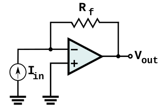
In electronics, a transimpedance amplifier (TIA) is a current to voltage converter, almost exclusively implemented with one or more operational amplifiers. The TIA can be used to amplify the current output of Geiger–Müller tubes, photo multiplier tubes, accelerometers, photo detectors and other types of sensors to a usable voltage. Current to voltage converters are used with sensors that have a current response that is more linear than the voltage response. This is the case with photodiodes where it is not uncommon for the current response to have better than 1% nonlinearity over a wide range of light input. The transimpedance amplifier presents a low impedance to the photodiode and isolates it from the output voltage of the operational amplifier. In its simplest form a transimpedance amplifier has just a large valued feedback resistor, R_f. The gain of the amplifier is set by this resistor and because the amplifier is in an inverting configuration, has a value of -R_f. There are several different configurations of transimpedance amplifiers, each suited to a particular application. The one factor they all have in common is the requirement to convert the low-level current of a sensor to a voltage. The gain, bandwidth, as well as current and voltage offsets change with different types of sensors, requiring different configurations of transimpedance amplifiers.

In geometry, the mean line segment length is the average length of a line segment connecting two points chosen uniformly at random in a given shape. In other words, it is the expected Euclidean distance between two random points, where each point in the shape is equally likely to be chosen.

References

Q.S. Wang, B.W. Yan, J. Planar Chromatogr. 9 (1996) 192.
B.J.M. de Spiegeleer, P.H.M. de Moerloose, G.A.S. Sleghers, Anal. Chem. 59 (1987) 62.
C.K. Bayne, C.Y. Ma, J. Liq. Chromatogr. 10 (1987) 3529.
S. Gocan, M. Mihaly, Stud Univ B-B Chemia, 1 (1991) 18.
S. Gocan, J. Planar Chromatogr. 4 (1991) 169.
Ł. Komsta, W. Markowski, G. Misztal, J. Planar Chromatogr. 20 (2007) 27.

Chromatographic response function

Contents

Examples in thin layer chromatography

Related Research Articles

References

See also