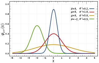
In probability theory and statistics, a normal distribution or Gaussian distribution is a type of continuous probability distribution for a real-valued random variable. The general form of its probability density function is The parameter is the mean or expectation of the distribution, while the parameter is the variance. The standard deviation of the distribution is (sigma). A random variable with a Gaussian distribution is said to be normally distributed, and is called a normal deviate.

In probability theory, a log-normal (or lognormal) distribution is a continuous probability distribution of a random variable whose logarithm is normally distributed. Thus, if the random variable X is log-normally distributed, then Y = ln(X) has a normal distribution. Equivalently, if Y has a normal distribution, then the exponential function of Y, X = exp(Y), has a log-normal distribution. A random variable which is log-normally distributed takes only positive real values. It is a convenient and useful model for measurements in exact and engineering sciences, as well as medicine, economics and other topics (e.g., energies, concentrations, lengths, prices of financial instruments, and other metrics).
In statistics, maximum likelihood estimation (MLE) is a method of estimating the parameters of an assumed probability distribution, given some observed data. This is achieved by maximizing a likelihood function so that, under the assumed statistical model, the observed data is most probable. The point in the parameter space that maximizes the likelihood function is called the maximum likelihood estimate. The logic of maximum likelihood is both intuitive and flexible, and as such the method has become a dominant means of statistical inference.

In statistical mechanics and information theory, the Fokker–Planck equation is a partial differential equation that describes the time evolution of the probability density function of the velocity of a particle under the influence of drag forces and random forces, as in Brownian motion. The equation can be generalized to other observables as well. The Fokker-Planck equation has multiple applications in information theory, graph theory, data science, finance, economics etc.
In probability theory and statistics, the cumulantsκn of a probability distribution are a set of quantities that provide an alternative to the moments of the distribution. Any two probability distributions whose moments are identical will have identical cumulants as well, and vice versa.
In probability theory, the Borel–Kolmogorov paradox is a paradox relating to conditional probability with respect to an event of probability zero. It is named after Émile Borel and Andrey Kolmogorov.

In biology, a substitution model, also called models of sequence evolution, are Markov models that describe changes over evolutionary time. These models describe evolutionary changes in macromolecules, such as DNA sequences or protein sequences, that can be represented as sequence of symbols. Substitution models are used to calculate the likelihood of phylogenetic trees using multiple sequence alignment data. Thus, substitution models are central to maximum likelihood estimation of phylogeny as well as Bayesian inference in phylogeny. Estimates of evolutionary distances are typically calculated using substitution models. Substitution models are also central to phylogenetic invariants because they are necessary to predict site pattern frequencies given a tree topology. Substitution models are also necessary to simulate sequence data for a group of organisms related by a specific tree.
In fluid dynamics, Couette flow is the flow of a viscous fluid in the space between two surfaces, one of which is moving tangentially relative to the other. The relative motion of the surfaces imposes a shear stress on the fluid and induces flow. Depending on the definition of the term, there may also be an applied pressure gradient in the flow direction.

Genetic distance is a measure of the genetic divergence between species or between populations within a species, whether the distance measures time from common ancestor or degree of differentiation. Populations with many similar alleles have small genetic distances. This indicates that they are closely related and have a recent common ancestor.
In queueing theory, a discipline within the mathematical theory of probability, a Jackson network is a class of queueing network where the equilibrium distribution is particularly simple to compute as the network has a product-form solution. It was the first significant development in the theory of networks of queues, and generalising and applying the ideas of the theorem to search for similar product-form solutions in other networks has been the subject of much research, including ideas used in the development of the Internet. The networks were first identified by James R. Jackson and his paper was re-printed in the journal Management Science’s ‘Ten Most Influential Titles of Management Sciences First Fifty Years.’
Bayesian inference of phylogeny combines the information in the prior and in the data likelihood to create the so-called posterior probability of trees, which is the probability that the tree is correct given the data, the prior and the likelihood model. Bayesian inference was introduced into molecular phylogenetics in the 1990s by three independent groups: Bruce Rannala and Ziheng Yang in Berkeley, Bob Mau in Madison, and Shuying Li in University of Iowa, the last two being PhD students at the time. The approach has become very popular since the release of the MrBayes software in 2001, and is now one of the most popular methods in molecular phylogenetics.
A number of different Markov models of DNA sequence evolution have been proposed. These substitution models differ in terms of the parameters used to describe the rates at which one nucleotide replaces another during evolution. These models are frequently used in molecular phylogenetic analyses. In particular, they are used during the calculation of likelihood of a tree and they are used to estimate the evolutionary distance between sequences from the observed differences between the sequences.
A ratio distribution is a probability distribution constructed as the distribution of the ratio of random variables having two other known distributions. Given two random variables X and Y, the distribution of the random variable Z that is formed as the ratio Z = X/Y is a ratio distribution.
In nonideal fluid dynamics, the Hagen–Poiseuille equation, also known as the Hagen–Poiseuille law, Poiseuille law or Poiseuille equation, is a physical law that gives the pressure drop in an incompressible and Newtonian fluid in laminar flow flowing through a long cylindrical pipe of constant cross section. It can be successfully applied to air flow in lung alveoli, or the flow through a drinking straw or through a hypodermic needle. It was experimentally derived independently by Jean Léonard Marie Poiseuille in 1838 and Gotthilf Heinrich Ludwig Hagen, and published by Hagen in 1839 and then by Poiseuille in 1840–41 and 1846. The theoretical justification of the Poiseuille law was given by George Stokes in 1845.
The auxiliary particle filter is a particle filtering algorithm introduced by Pitt and Shephard in 1999 to improve some deficiencies of the sequential importance resampling (SIR) algorithm when dealing with tailed observation densities.

In probability theory, a logit-normal distribution is a probability distribution of a random variable whose logit has a normal distribution. If Y is a random variable with a normal distribution, and t is the standard logistic function, then X = t(Y) has a logit-normal distribution; likewise, if X is logit-normally distributed, then Y = logit(X)= log (X/(1-X)) is normally distributed. It is also known as the logistic normal distribution, which often refers to a multinomial logit version (e.g.).
Stochastic portfolio theory (SPT) is a mathematical theory for analyzing stock market structure and portfolio behavior introduced by E. Robert Fernholz in 2002. It is descriptive as opposed to normative, and is consistent with the observed behavior of actual markets. Normative assumptions, which serve as a basis for earlier theories like modern portfolio theory (MPT) and the capital asset pricing model (CAPM), are absent from SPT.
In machine learning, the kernel embedding of distributions comprises a class of nonparametric methods in which a probability distribution is represented as an element of a reproducing kernel Hilbert space (RKHS). A generalization of the individual data-point feature mapping done in classical kernel methods, the embedding of distributions into infinite-dimensional feature spaces can preserve all of the statistical features of arbitrary distributions, while allowing one to compare and manipulate distributions using Hilbert space operations such as inner products, distances, projections, linear transformations, and spectral analysis. This learning framework is very general and can be applied to distributions over any space on which a sensible kernel function may be defined. For example, various kernels have been proposed for learning from data which are: vectors in , discrete classes/categories, strings, graphs/networks, images, time series, manifolds, dynamical systems, and other structured objects. The theory behind kernel embeddings of distributions has been primarily developed by Alex Smola, Le Song , Arthur Gretton, and Bernhard Schölkopf. A review of recent works on kernel embedding of distributions can be found in.
In statistics, the variance function is a smooth function that depicts the variance of a random quantity as a function of its mean. The variance function is a measure of heteroscedasticity and plays a large role in many settings of statistical modelling. It is a main ingredient in the generalized linear model framework and a tool used in non-parametric regression, semiparametric regression and functional data analysis. In parametric modeling, variance functions take on a parametric form and explicitly describe the relationship between the variance and the mean of a random quantity. In a non-parametric setting, the variance function is assumed to be a smooth function.
In physics and mathematics, the Klein–Kramers equation or sometimes referred as Kramers–Chandrasekhar equation is a partial differential equation that describes the probability density function f of a Brownian particle in phase space (r, p). It is a special case of the Fokker–Planck equation.


