Differential equations arise in many problems in physics, engineering, and other sciences. The following examples show how to solve differential equations in a few simple cases when an exact solution exists.

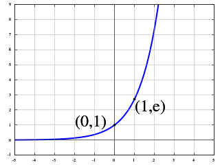
In mathematics, an exponential function is a function of the form

The heat equation is a parabolic partial differential equation that describes the distribution of heat in a given region over time.
The ordered exponential, also called the path-ordered exponential, is a mathematical operation defined in non-commutative algebras, equivalent to the exponential of the integral in the commutative algebras. In practice the ordered exponential is used in matrix and operator algebras.
In mathematics, a linear differential equation is a differential equation that is defined by a linear polynomial in the unknown function and its derivatives, that is an equation of the form
The Lotka–Volterra equations, also known as the predator–prey equations, are a pair of first-order nonlinear differential equations, frequently used to describe the dynamics of biological systems in which two species interact, one as a predator and the other as prey. The populations change through time according to the pair of equations:
In mathematics and its applications, a classical Sturm–Liouville theory, named after Jacques Charles François Sturm (1803–1855) and Joseph Liouville (1809–1882), is the theory of a real second-order linear differential equation of the form
In mathematics, the matrix exponential is a matrix function on square matrices analogous to the ordinary exponential function. It is used to solve systems of linear differential equations. In the theory of Lie groups, the matrix exponential gives the connection between a matrix Lie algebra and the corresponding Lie group.
In mathematical physics, the WKB approximation or WKB method is a method for finding approximate solutions to linear differential equations with spatially varying coefficients. It is typically used for a semiclassical calculation in quantum mechanics in which the wavefunction is recast as an exponential function, semiclassically expanded, and then either the amplitude or the phase is taken to be changing slowly.
In mathematics and particularly in dynamic systems, an initial condition, in some contexts called a seed value, is a value of an evolving variable at some point in time designated as the initial time. For a system of order k and dimension n, generally nk initial conditions are needed in order to trace the system's variables forward through time.

In applied mathematics, in particular the context of nonlinear system analysis, a phase plane is a visual display of certain characteristics of certain kinds of differential equations; a coordinate plane with axes being the values of the two state variables, say, or etc.. It is a two-dimensional case of the general n-dimensional phase space.
Reduction of order is a technique in mathematics for solving second-order linear ordinary differential equations. It is employed when one solution is known and a second linearly independent solution is desired. The method also applies to n-th order equations. In this case the ansatz will yield an (n-1)-th order equation for .

In physics, Hamilton's principle is William Rowan Hamilton's formulation of the principle of stationary action. It states that the dynamics of a physical system is determined by a variational problem for a functional based on a single function, the Lagrangian, which contains all physical information concerning the system and the forces acting on it. The variational problem is equivalent to and allows for the derivation of the differential equations of motion of the physical system. Although formulated originally for classical mechanics, Hamilton's principle also applies to classical fields such as the electromagnetic and gravitational fields, and plays an important role in quantum mechanics, quantum field theory and criticality theories.
In theory of vibrations, Duhamel's integral is a way of calculating the response of linear systems and structures to arbitrary time-varying external perturbation.
A parabolic partial differential equation is a type of partial differential equation (PDE). Parabolic PDEs are used to describe a wide variety of time-dependent phenomena, including heat conduction, particle diffusion, and pricing of derivative investment instruments.
In stochastic calculus, the Doléans-Dade exponential, Doléans exponential, or stochastic exponential, of a semimartingale X is defined to be the solution to the stochastic differential equation dYt = Yt dXt with initial condition Y0 = 1. The concept is named after Catherine Doléans-Dade. It is sometimes denoted by Ɛ(X). In the case where X is differentiable, then Y is given by the differential equation dY/dt = Y dX/dt to which the solution is Y = exp(X − X0). Alternatively, if Xt = σBt + μt for a Brownian motion B, then the Doléans-Dade exponential is a geometric Brownian motion. For any continuous semimartingale X, applying Itō's lemma with ƒ(Y) = log(Y) gives
In mathematics and physics, the Magnus expansion, named after Wilhelm Magnus (1907–1990), provides an exponential representation of the solution of a first order homogeneous linear differential equation for a linear operator. In particular it furnishes the fundamental matrix of a system of linear ordinary differential equations of order n with varying coefficients. The exponent is aggregated as an infinite series whose terms involve multiple integrals and nested commutators.
In mathematics, the slow manifold of an equilibrium point of a dynamical system occurs as the most common example of a center manifold. One of the main methods of simplifying dynamical systems, is to reduce the dimension of the system to that of the slow manifold—center manifold theory rigorously justifies the modelling. For example, some global and regional models of the atmosphere or oceans resolve the so-called quasi-geostrophic flow dynamics on the slow manifold of the atmosphere/oceanic dynamics, and is thus crucial to forecasting with a climate model.

In mathematics, the exponential response formula (ERF), also known as exponential response and complex replacement, is a method used to find a particular solution of a non-homogeneous linear ordinary differential equation of any order. The exponential response formula is applicable to non-homogeneous linear ordinary differential equations with constant coefficients if the function is polynomial, sinusoidal, exponential or the combination of the three. The general solution of a non-homogeneous linear ordinary differential equation is a superposition of the general solution of the associated homogeneous ODE and a particular solution to the non-homogeneous ODE. Alternative methods for solving ordinary differential equations of higher order are method of undetermined coefficients and method of variation of parameters.


