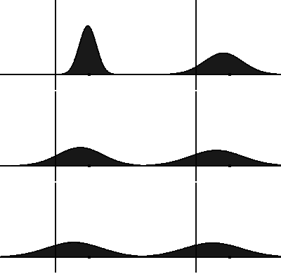
A Markov chain or Markov process is a stochastic model describing a sequence of possible events in which the probability of each event depends only on the state attained in the previous event. Informally, this may be thought of as, "What happens next depends only on the state of affairs now." A countably infinite sequence, in which the chain moves state at discrete time steps, gives a discrete-time Markov chain (DTMC). A continuous-time process is called a continuous-time Markov chain (CTMC). It is named after the Russian mathematician Andrey Markov.
In physics, a Langevin equation is a stochastic differential equation describing how a system evolves when subjected to a combination of deterministic and fluctuating ("random") forces. The dependent variables in a Langevin equation typically are collective (macroscopic) variables changing only slowly in comparison to the other (microscopic) variables of the system. The fast (microscopic) variables are responsible for the stochastic nature of the Langevin equation. One application is to Brownian motion, which models the fluctuating motion of a small particle in a fluid.

In statistical mechanics and information theory, the Fokker–Planck equation is a partial differential equation that describes the time evolution of the probability density function of the velocity of a particle under the influence of drag forces and random forces, as in Brownian motion. The equation can be generalized to other observables as well. The Fokker-Planck equation has multiple applications in information theory, graph theory, data science, finance, economics etc.
In mathematics, a stochastic matrix is a square matrix used to describe the transitions of a Markov chain. Each of its entries is a nonnegative real number representing a probability. It is also called a probability matrix, transition matrix, substitution matrix, or Markov matrix. The stochastic matrix was first developed by Andrey Markov at the beginning of the 20th century, and has found use throughout a wide variety of scientific fields, including probability theory, statistics, mathematical finance and linear algebra, as well as computer science and population genetics. There are several different definitions and types of stochastic matrices:

In probability theory and statistics, the term Markov property refers to the memoryless property of a stochastic process, which means that its future evolution is independent of its history. It is named after the Russian mathematician Andrey Markov. The term strong Markov property is similar to the Markov property, except that the meaning of "present" is defined in terms of a random variable known as a stopping time.
In mathematics, the covariant derivative is a way of specifying a derivative along tangent vectors of a manifold. Alternatively, the covariant derivative is a way of introducing and working with a connection on a manifold by means of a differential operator, to be contrasted with the approach given by a principal connection on the frame bundle – see affine connection. In the special case of a manifold isometrically embedded into a higher-dimensional Euclidean space, the covariant derivative can be viewed as the orthogonal projection of the Euclidean directional derivative onto the manifold's tangent space. In this case the Euclidean derivative is broken into two parts, the extrinsic normal component and the intrinsic covariant derivative component.
In physics, chemistry, and related fields, master equations are used to describe the time evolution of a system that can be modeled as being in a probabilistic combination of states at any given time, and the switching between states is determined by a transition rate matrix. The equations are a set of differential equations – over time – of the probabilities that the system occupies each of the different states.
The Lyapunov equation, named after the Russian mathematician Aleksandr Lyapunov, is a matrix equation used in the stability analysis of linear dynamical systems.
In differential geometry, the four-gradient is the four-vector analogue of the gradient from vector calculus.
A mathematical or physical process is time-reversible if the dynamics of the process remain well-defined when the sequence of time-states is reversed.

In mathematics, the Ornstein–Uhlenbeck process is a stochastic process with applications in financial mathematics and the physical sciences. Its original application in physics was as a model for the velocity of a massive Brownian particle under the influence of friction. It is named after Leonard Ornstein and George Eugene Uhlenbeck.
The theoretical and experimental justification for the Schrödinger equation motivates the discovery of the Schrödinger equation, the equation that describes the dynamics of nonrelativistic particles. The motivation uses photons, which are relativistic particles with dynamics described by Maxwell's equations, as an analogue for all types of particles.
The derivation of the Navier–Stokes equations as well as their application and formulation for different families of fluids, is an important exercise in fluid dynamics with applications in mechanical engineering, physics, chemistry, heat transfer, and electrical engineering. A proof explaining the properties and bounds of the equations, such as Navier–Stokes existence and smoothness, is one of the important unsolved problems in mathematics.
The discrete phase-type distribution is a probability distribution that results from a system of one or more inter-related geometric distributions occurring in sequence, or phases. The sequence in which each of the phases occur may itself be a stochastic process. The distribution can be represented by a random variable describing the time until absorption of an absorbing Markov chain with one absorbing state. Each of the states of the Markov chain represents one of the phases.
In mathematics – specifically, in stochastic analysis – an Itô diffusion is a solution to a specific type of stochastic differential equation. That equation is similar to the Langevin equation used in physics to describe the Brownian motion of a particle subjected to a potential in a viscous fluid. Itô diffusions are named after the Japanese mathematician Kiyosi Itô.
The Cauchy momentum equation is a vector partial differential equation put forth by Cauchy that describes the non-relativistic momentum transport in any continuum.
In probability theory, Kolmogorov equations, including Kolmogorov forward equations and Kolmogorov backward equations, characterize continuous-time Markov processes. In particular, they describe how the probability of a continuous-time Markov process in a certain state changes over time.

In dynamics, probability, physics, chemistry and related fields, a heterogeneous random walk in one dimension is a random walk in a one dimensional interval with jumping rules that depend on the location of the random walker in the interval.
In mathematics, specifically in the theory of Markovian stochastic processes in probability theory, the Chapman–Kolmogorov equation (CKE) is an identity relating the joint probability distributions of different sets of coordinates on a stochastic process. The equation was derived independently by both the British mathematician Sydney Chapman and the Russian mathematician Andrey Kolmogorov. The CKE is prominently used in recent Variational Bayesian methods.
In stochastic processes, Kramers–Moyal expansion refers to a Taylor series expansion of the master equation, named after Hans Kramers and José Enrique Moyal. In many textbooks, the expansion is used only to derive the Fokker–Planck equation, and never used again. In general, continuous stochastic processes are essentially all Markovian, and so Fokker–Planck equations are sufficient for studying them. The higher-order Kramers–Moyal expansion only come into play when the process is jumpy. This usually means it is a Poisson-like process.


