Control theory in control systems engineering is a subfield of mathematics that deals with the control of continuously operating dynamical systems in engineered processes and machines. The objective is to develop a control model for controlling such systems using a control action in an optimum manner without delay or overshoot and ensuring control stability.

Artificial neural networks (ANN) or connectionist systems are computing systems vaguely inspired by the biological neural networks that constitute animal brains. The neural network itself is not an algorithm, but rather a framework for many different machine learning algorithms to work together and process complex data inputs. Such systems "learn" to perform tasks by considering examples, generally without being programmed with any task-specific rules. For example, in image recognition, they might learn to identify images that contain cats by analyzing example images that have been manually labeled as "cat" or "no cat" and using the results to identify cats in other images. They do this without any prior knowledge about cats, for example, that they have fur, tails, whiskers and cat-like faces. Instead, they automatically generate identifying characteristics from the learning material that they process.
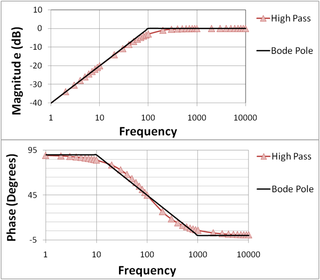
In electrical engineering and control theory, a Bode plot is a graph of the frequency response of a system. It is usually a combination of a Bode magnitude plot, expressing the magnitude of the frequency response, and a Bode phase plot, expressing the phase shift.
In computer programming, a parameter or a formal argument, is a special kind of variable, used in a subroutine to refer to one of the pieces of data provided as input to the subroutine. These pieces of data are the values of the arguments with which the subroutine is going to be called/invoked. An ordered list of parameters is usually included in the definition of a subroutine, so that, each time the subroutine is called, its arguments for that call are evaluated, and the resulting values can be assigned to the corresponding parameters.
An artificial neuron is a mathematical function conceived as a model of biological neurons, a neural network. Artificial neurons are elementary units in an artificial neural network. The artificial neuron receives one or more inputs and sums them to produce an output. Usually each input is separately weighted, and the sum is passed through a non-linear function known as an activation function or transfer function. The transfer functions usually have a sigmoid shape, but they may also take the form of other non-linear functions, piecewise linear functions, or step functions. They are also often monotonically increasing, continuous, differentiable and bounded. The thresholding function has inspired building logic gates referred to as threshold logic; applicable to building logic circuits resembling brain processing. For example, new devices such as memristors have been extensively used to develop such logic in recent times.
Digital control is a branch of control theory that uses digital computers to act as system controllers. Depending on the requirements, a digital control system can take the form of a microcontroller to an ASIC to a standard desktop computer. Since a digital computer is a discrete system, the Laplace transform is replaced with the Z-transform. Also since a digital computer has finite precision, extra care is needed to ensure the error in coefficients, A/D conversion, D/A conversion, etc. are not producing undesired or unplanned effects.

The superposition principle, also known as superposition property, states that, for all linear systems, the net response caused by two or more stimuli is the sum of the responses that would have been caused by each stimulus individually. So that if input A produces response X and input B produces response Y then input produces response.
Linear time-invariant theory, commonly known as LTI system theory, comes from applied mathematics and has direct applications in NMR spectroscopy, seismology, circuits, signal processing, control theory, and other technical areas. It investigates the response of a linear and time-invariant system to an arbitrary input signal. Trajectories of these systems are commonly measured and tracked as they move through time, but in applications like image processing and field theory, the LTI systems also have trajectories in spatial dimensions. Thus, these systems are also called linear translation-invariant to give the theory the most general reach. In the case of generic discrete-time systems, linear shift-invariant is the corresponding term. A good example of LTI systems are electrical circuits that can be made up of resistors, capacitors, and inductors.

In probability theory and statistics, the continuous uniform distribution or rectangular distribution is a family of symmetric probability distributions such that for each member of the family, all intervals of the same length on the distribution's support are equally probable. The support is defined by the two parameters, a and b, which are its minimum and maximum values. The distribution is often abbreviated U(a,b). It is the maximum entropy probability distribution for a random variable X under no constraint other than that it is contained in the distribution's support.
In computability theory the smn theorem, is a basic result about programming languages. It was first proved by Stephen Cole Kleene (1943). The name "smn" comes from the occurrence of a s with subscript n and superscript m in the original formulation of the theorem.

In mathematics a Padé approximant is the 'best' approximation of a function by a rational function of given order – under this technique, the approximant's power series agrees with the power series of the function it is approximating. The technique was developed around 1890 by Henri Padé, but goes back to Georg Frobenius who introduced the idea and investigated the features of rational approximations of power series.
Uncertainty quantification (UQ) is the science of quantitative characterization and reduction of uncertainties in both computational and real world applications. It tries to determine how likely certain outcomes are if some aspects of the system are not exactly known. An example would be to predict the acceleration of a human body in a head-on crash with another car: even if we exactly knew the speed, small differences in the manufacturing of individual cars, how tightly every bolt has been tightened, etc., will lead to different results that can only be predicted in a statistical sense.
The beam propagation method (BPM) is an approximation technique for simulating the propagation of light in slowly varying optical waveguides. It is essentially the same as the so-called parabolic equation (PE) method in underwater acoustics. Both BPM and the PE were first introduced in the 1970s. When a wave propagates along a waveguide for a large distance, rigorous numerical simulation is difficult. The BPM relies on approximate differential equations which are also called the one-way models. These one-way models involve only a first order derivative in the variable z and they can be solved as "initial" value problem. The "initial" value problem does not involve time, rather it is for the spatial variable z.
In the field of mathematical modeling, a radial basis function network is an artificial neural network that uses radial basis functions as activation functions. The output of the network is a linear combination of radial basis functions of the inputs and neuron parameters. Radial basis function networks have many uses, including function approximation, time series prediction, classification, and system control. They were first formulated in a 1988 paper by Broomhead and Lowe, both researchers at the Royal Signals and Radar Establishment.

In statistics, the Q-function is the tail distribution function of the standard normal distribution. In other words, is the probability that a normal (Gaussian) random variable will obtain a value larger than standard deviations. Equivalently, is the probability that a standard normal random variable takes a value larger than .

Advanced process monitor (APMonitor), is a modeling language for differential algebraic (DAE) equations. It is a free web-service or local server for solving representations of physical systems in the form of implicit DAE models. APMonitor is suited for large-scale problems and solves linear programming, integer programming, nonlinear programming, nonlinear mixed integer programming, dynamic simulation, moving horizon estimation, and nonlinear model predictive control. APMonitor does not solve the problems directly, but calls nonlinear programming solvers such as APOPT, BPOPT, IPOPT, MINOS, and SNOPT. The APMonitor API provides exact first and second derivatives of continuous functions to the solvers through automatic differentiation and in sparse matrix form.

The finite element method (FEM), is a numerical method for solving problems of engineering and mathematical physics. Typical problem areas of interest include structural analysis, heat transfer, fluid flow, mass transport, and electromagnetic potential. The analytical solution of these problems generally require the solution to boundary value problems for partial differential equations. The finite element method formulation of the problem results in a system of algebraic equations. The method approximates the unknown function over the domain. To solve the problem, it subdivides a large system into smaller, simpler parts that are called finite elements. The simple equations that model these finite elements are then assembled into a larger system of equations that models the entire problem. FEM then uses variational methods from the calculus of variations to approximate a solution by minimizing an associated error function.
System identification is a method of identifying or measuring the mathematical model of a system from measurements of the system inputs and outputs. The applications of system identification include any system where the inputs and outputs can be measured and include industrial processes, control systems, economic data, biology and the life sciences, medicine, social systems and many more.
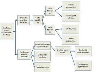
Simulation-based optimization integrates optimization techniques into simulation analysis. Because of the complexity of the simulation, the objective function may become difficult and expensive to evaluate.


