
Ḥasan Ibn al-Haytham was a medieval mathematician, astronomer, and physicist of the Islamic Golden Age from present-day Iraq. Referred to as "the father of modern optics", he made significant contributions to the principles of optics and visual perception in particular. His most influential work is titled Kitāb al-Manāẓir, written during 1011–1021, which survived in a Latin edition. The works of Alhazen were frequently cited during the scientific revolution by Isaac Newton, Johannes Kepler, Christiaan Huygens, and Galileo Galilei.

Lambda is the eleventh letter of the Greek alphabet, representing the voiced alveolar lateral approximant IPA:[l]. In the system of Greek numerals, lambda has a value of 30. Lambda is derived from the Phoenician Lamed. Lambda gave rise to the Latin L and the Cyrillic El (Л). The ancient grammarians and dramatists give evidence to the pronunciation as (λάβδα) in Classical Greek times. In Modern Greek, the name of the letter, Λάμδα, is pronounced.
Ray transfer matrix analysis is a mathematical form for performing ray tracing calculations in sufficiently simple problems which can be solved considering only paraxial rays. Each optical element is described by a 2 × 2ray transfer matrix which operates on a vector describing an incoming light ray to calculate the outgoing ray. Multiplication of the successive matrices thus yields a concise ray transfer matrix describing the entire optical system. The same mathematics is also used in accelerator physics to track particles through the magnet installations of a particle accelerator, see electron optics.
An inverse problem in science is the process of calculating from a set of observations the causal factors that produced them: for example, calculating an image in X-ray computed tomography, source reconstruction in acoustics, or calculating the density of the Earth from measurements of its gravity field. It is called an inverse problem because it starts with the effects and then calculates the causes. It is the inverse of a forward problem, which starts with the causes and then calculates the effects.

Specular reflection, or regular reflection, is the mirror-like reflection of waves, such as light, from a surface.

In physics, physical optics, or wave optics, is the branch of optics that studies interference, diffraction, polarization, and other phenomena for which the ray approximation of geometric optics is not valid. This usage tends not to include effects such as quantum noise in optical communication, which is studied in the sub-branch of coherence theory.

In geometric optics, the paraxial approximation is a small-angle approximation used in Gaussian optics and ray tracing of light through an optical system.
Nonimaging optics is a branch of optics that is concerned with the optimal transfer of light radiation between a source and a target. Unlike traditional imaging optics, the techniques involved do not attempt to form an image of the source; instead an optimized optical system for optimal radiative transfer from a source to a target is desired.

In optics, a ray is an idealized geometrical model of light or other electromagnetic radiation, obtained by choosing a curve that is perpendicular to the wavefronts of the actual light, and that points in the direction of energy flow. Rays are used to model the propagation of light through an optical system, by dividing the real light field up into discrete rays that can be computationally propagated through the system by the techniques of ray tracing. This allows even very complex optical systems to be analyzed mathematically or simulated by computer. Ray tracing uses approximate solutions to Maxwell's equations that are valid as long as the light waves propagate through and around objects whose dimensions are much greater than the light's wavelength. Ray optics or geometrical optics does not describe phenomena such as diffraction, which require wave optics theory. Some wave phenomena such as interference can be modeled in limited circumstances by adding phase to the ray model.

Computational electromagnetics (CEM), computational electrodynamics or electromagnetic modeling is the process of modeling the interaction of electromagnetic fields with physical objects and the environment using computers.
In physics, ray tracing is a method for calculating the path of waves or particles through a system with regions of varying propagation velocity, absorption characteristics, and reflecting surfaces. Under these circumstances, wavefronts may bend, change direction, or reflect off surfaces, complicating analysis.
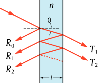
The transfer-matrix method is a method used in optics and acoustics to analyze the propagation of electromagnetic or acoustic waves through a stratified medium; a stack of thin films. This is, for example, relevant for the design of anti-reflective coatings and dielectric mirrors.
Beam expanders are optical devices that take a collimated beam of light and expand its width.

In mathematics, a matrix is a rectangular array or table of numbers, symbols, or expressions, with elements or entries arranged in rows and columns, which is used to represent a mathematical object or property of such an object.

Optics is a work on the geometry of vision written by the Greek mathematician Euclid around 300 BC. The earliest surviving manuscript of Optics is in Greek and dates from the 10th century AD.
The Transition Matrix Method is a computational technique of light scattering by nonspherical particles originally formulated by Peter C. Waterman (1928–2012) in 1965. The technique is also known as null field method and extended boundary condition method (EBCM). In the method, matrix elements are obtained by matching boundary conditions for solutions of Maxwell equations. It has been greatly extended to incorporate diverse types of linear media occupying the region enclosing the scatterer. T-matrix method proves to be highly efficient and has been widely used in computing electromagnetic scattering of single and compound particles.
OPTOS is a simulation formalism for determining optical properties of sheets with plane-parallel structured interfaces. The method is versatile as interface structures of different optical regimes, e.g. geometrical and wave optics, can be included. It is very efficient due to the re-usability of the calculated light redistribution properties of the individual interfaces. It has so far been mainly used to model optical properties of solar cells and solar modules but it is also applicable for example to LEDs or OLEDs with light extraction structures.
Florin Abelès was a French physicist, specialized in optics.