In mathematics, and more specifically in linear algebra, a linear map is a mapping between two vector spaces that preserves the operations of vector addition and scalar multiplication. The same names and the same definition are also used for the more general case of modules over a ring; see Module homomorphism.

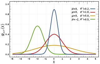
In probability theory and statistics, a normal distribution or Gaussian distribution is a type of continuous probability distribution for a real-valued random variable. The general form of its probability density function is The parameter is the mean or expectation of the distribution, while the parameter is the variance. The standard deviation of the distribution is . A random variable with a Gaussian distribution is said to be normally distributed, and is called a normal deviate.
A likelihood function measures how well a statistical model explains observed data by calculating the probability of seeing that data under different parameter values of the model. It is constructed from the joint probability distribution of the random variable that (presumably) generated the observations. When evaluated on the actual data points, it becomes a function solely of the model parameters.

In probability theory and statistics, the negative binomial distribution is a discrete probability distribution that models the number of failures in a sequence of independent and identically distributed Bernoulli trials before a specified (non-random) number of successes occurs. For example, we can define rolling a 6 on some dice as a success, and rolling any other number as a failure, and ask how many failure rolls will occur before we see the third success. In such a case, the probability distribution of the number of failures that appear will be a negative binomial distribution.
Reed–Solomon codes are a group of error-correcting codes that were introduced by Irving S. Reed and Gustave Solomon in 1960. They have many applications, including consumer technologies such as MiniDiscs, CDs, DVDs, Blu-ray discs, QR codes, Data Matrix, data transmission technologies such as DSL and WiMAX, broadcast systems such as satellite communications, DVB and ATSC, and storage systems such as RAID 6.
In mathematical optimization, the method of Lagrange multipliers is a strategy for finding the local maxima and minima of a function subject to equation constraints. It is named after the mathematician Joseph-Louis Lagrange.
In physics, the CHSH inequality can be used in the proof of Bell's theorem, which states that certain consequences of entanglement in quantum mechanics cannot be reproduced by local hidden-variable theories. Experimental verification of the inequality being violated is seen as confirmation that nature cannot be described by such theories. CHSH stands for John Clauser, Michael Horne, Abner Shimony, and Richard Holt, who described it in a much-cited paper published in 1969. They derived the CHSH inequality, which, as with John Stewart Bell's original inequality, is a constraint—on the statistical occurrence of "coincidences" in a Bell test—which is necessarily true if an underlying local hidden-variable theory exists. In practice, the inequality is routinely violated by modern experiments in quantum mechanics.
The principle of maximum entropy states that the probability distribution which best represents the current state of knowledge about a system is the one with largest entropy, in the context of precisely stated prior data.
In the theory of stochastic processes, the Karhunen–Loève theorem, also known as the Kosambi–Karhunen–Loève theorem states that a stochastic process can be represented as an infinite linear combination of orthogonal functions, analogous to a Fourier series representation of a function on a bounded interval. The transformation is also known as Hotelling transform and eigenvector transform, and is closely related to principal component analysis (PCA) technique widely used in image processing and in data analysis in many fields.
In probability theory, a compound Poisson distribution is the probability distribution of the sum of a number of independent identically-distributed random variables, where the number of terms to be added is itself a Poisson-distributed variable. The result can be either a continuous or a discrete distribution.
In mathematics, the discrete Laplace operator is an analog of the continuous Laplace operator, defined so that it has meaning on a graph or a discrete grid. For the case of a finite-dimensional graph, the discrete Laplace operator is more commonly called the Laplacian matrix.
In probability theory and mathematical physics, a random matrix is a matrix-valued random variable—that is, a matrix in which some or all of its entries are sampled randomly from a probability distribution. Random matrix theory (RMT) is the study of properties of random matrices, often as they become large. RMT provides techniques like mean-field theory, diagrammatic methods, the cavity method, or the replica method to compute quantities like traces, spectral densities, or scalar products between eigenvectors. Many physical phenomena, such as the spectrum of nuclei of heavy atoms, the thermal conductivity of a lattice, or the emergence of quantum chaos, can be modeled mathematically as problems concerning large, random matrices.
In statistics and information theory, a maximum entropy probability distribution has entropy that is at least as great as that of all other members of a specified class of probability distributions. According to the principle of maximum entropy, if nothing is known about a distribution except that it belongs to a certain class, then the distribution with the largest entropy should be chosen as the least-informative default. The motivation is twofold: first, maximizing entropy minimizes the amount of prior information built into the distribution; second, many physical systems tend to move towards maximal entropy configurations over time.
In the mathematical discipline of graph theory, the expander walk sampling theorem intuitively states that sampling vertices in an expander graph by doing relatively short random walk can simulate sampling the vertices independently from a uniform distribution. The earliest version of this theorem is due to Ajtai, Komlós & Szemerédi (1987), and the more general version is typically attributed to Gillman (1998).
In mathematics, the Prékopa–Leindler inequality is an integral inequality closely related to the reverse Young's inequality, the Brunn–Minkowski inequality and a number of other important and classical inequalities in analysis. The result is named after the Hungarian mathematicians András Prékopa and László Leindler.
In mathematics and theoretical physics, Noether's second theorem relates symmetries of an action functional with a system of differential equations. The theorem is named after its discoverer, Emmy Noether.

In probability theory and statistics, the Poisson distribution is a discrete probability distribution that expresses the probability of a given number of events occurring in a fixed interval of time if these events occur with a known constant mean rate and independently of the time since the last event. It can also be used for the number of events in other types of intervals than time, and in dimension greater than 1.
In probability theory and statistics, Campbell's theorem or the Campbell–Hardy theorem is either a particular equation or set of results relating to the expectation of a function summed over a point process to an integral involving the mean measure of the point process, which allows for the calculation of expected value and variance of the random sum. One version of the theorem, also known as Campbell's formula, entails an integral equation for the aforementioned sum over a general point process, and not necessarily a Poisson point process. There also exist equations involving moment measures and factorial moment measures that are considered versions of Campbell's formula. All these results are employed in probability and statistics with a particular importance in the theory of point processes and queueing theory as well as the related fields stochastic geometry, continuum percolation theory, and spatial statistics.

In probability theory, statistics and related fields, a Poisson point process is a type of mathematical object that consists of points randomly located on a mathematical space with the essential feature that the points occur independently of one another. The process's name derives from the fact that the distribution of the number of points regions of the same size has a Poisson distribution. The process and the distribution are named after French mathematician Siméon Denis Poisson. The process itself was discovered independently and repeatedly in several settings, including experiments on radioactive decay, telephone call arrivals and actuarial science.
Maximal entropy random walk (MERW) is a popular type of biased random walk on a graph, in which transition probabilities are chosen accordingly to the principle of maximum entropy, which says that the probability distribution which best represents the current state of knowledge is the one with largest entropy. While standard random walk chooses for every vertex uniform probability distribution among its outgoing edges, locally maximizing entropy rate, MERW maximizes it globally by assuming uniform probability distribution among all paths in a given graph.


