In economics, the Gini coefficient, sometimes called Gini index, or Gini ratio, is a measure of statistical dispersion intended to represent the income or wealth distribution of a nation's residents, and is the most commonly used measurement of inequality. It was developed by the Italian statistician and sociologist Corrado Gini and published in his 1912 paper Variability and Mutability.

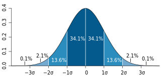
In statistics, the standard deviation is a measure that is used to quantify the amount of variation or dispersion of a set of data values. A low standard deviation indicates that the data points tend to be close to the mean of the set, while a high standard deviation indicates that the data points are spread out over a wider range of values.

In statistics, dependence or association is any statistical relationship, whether causal or not, between two random variables or bivariate data. In the broadest sense correlation is any statistical association, though in common usage it most often refers to how close two variables are to having a linear relationship with each other. Familiar examples of dependent phenomena include the correlation between the physical statures of parents and their offspring, and the correlation between the demand for a limited supply product and its price.

In statistics, the Pearson correlation coefficient, also referred to as Pearson's r, the Pearson product-moment correlation coefficient (PPMCC) or the bivariate correlation, is a measure of the linear correlation between two variables X and Y. According to the Cauchy–Schwarz inequality it has a value between +1 and −1, where 1 is total positive linear correlation, 0 is no linear correlation, and −1 is total negative linear correlation. It is widely used in the sciences. It was developed by Karl Pearson from a related idea introduced by Francis Galton in the 1880s and for which the mathematical formula was derived and published by Auguste Bravais in 1844.. The naming of the coefficient is thus an example of Stigler's Law.

In statistics, the standard score is the signed fractional number of standard deviations by which the value of an observation or data point is above the mean value of what is being observed or measured. Observed values above the mean have positive standard scores, while values below the mean have negative standard scores.

In statistics, Spearman's rank correlation coefficient or Spearman's rho, named after Charles Spearman and often denoted by the Greek letter (rho) or as , is a nonparametric measure of rank correlation. It assesses how well the relationship between two variables can be described using a monotonic function.
The Mahalanobis distance is a measure of the distance between a point P and a distribution D, introduced by P. C. Mahalanobis in 1936. It is a multi-dimensional generalization of the idea of measuring how many standard deviations away P is from the mean of D. This distance is zero if P is at the mean of D, and grows as P moves away from the mean along each principal component axis. The Mahalanobis distance measures the number of standard deviations from P to the mean of D. If each of these axes is re-scaled to have unit variance, then the Mahalanobis distance corresponds to standard Euclidean distance in the transformed space. The Mahalanobis distance is thus unitless and scale-invariant, and takes into account the correlations of the data set.
In probability theory and statistics, the coefficient of variation (CV), also known as relative standard deviation (RSD), is a standardized measure of dispersion of a probability distribution or frequency distribution. It is often expressed as a percentage, and is defined as the ratio of the standard deviation to the mean . The CV or RSD is widely used in analytical chemistry to express the precision and repeatability of an assay. It is also commonly used in fields such as engineering or physics when doing quality assurance studies and ANOVA gauge R&R. In addition, CV is utilized by economists and investors in economic models and in determining the volatility of a security.

In statistics, a bimodal distribution is a continuous probability distribution with two different modes. These appear as distinct peaks in the probability density function, as shown in Figures 1 and 2.

In statistics, the coefficient of determination, denoted R2 or r2 and pronounced "R squared", is the proportion of the variance in the dependent variable that is predictable from the independent variable(s).
Most of the terms listed in Wikipedia glossaries are already defined and explained within Wikipedia itself. However, glossaries like this one are useful for looking up, comparing and reviewing large numbers of terms together. You can help enhance this page by adding new terms or writing definitions for existing ones.

In statistics, simple linear regression is a linear regression model with a single explanatory variable. That is, it concerns two-dimensional sample points with one independent variable and one dependent variable and finds a linear function that, as accurately as possible, predicts the dependent variable values as a function of the independent variables. The adjective simple refers to the fact that the outcome variable is related to a single predictor.
The point biserial correlation coefficient (rpb) is a correlation coefficient used when one variable is dichotomous; Y can either be "naturally" dichotomous, like whether a coin lands heads or tails, or an artificially dichotomized variable. In most situations it is not advisable to dichotomize variables artificially. When a new variable is artificially dichotomized the new dichotomous variable may be conceptualized as having an underlying continuity. If this is the case, a biserial correlation would be the more appropriate calculation.
The root-mean-square deviation (RMSD) or root-mean-square error (RMSE) is a frequently used measure of the differences between values predicted by a model or an estimator and the values observed. The RMSD represents the square root of the second sample moment of the differences between predicted values and observed values or the quadratic mean of these differences. These deviations are called residuals when the calculations are performed over the data sample that was used for estimation and are called errors when computed out-of-sample. The RMSD serves to aggregate the magnitudes of the errors in predictions for various times into a single measure of predictive power. RMSD is a measure of accuracy, to compare forecasting errors of different models for a particular dataset and not between datasets, as it is scale-dependent.
In probability theory and statistics, partial correlation measures the degree of association between two random variables, with the effect of a set of controlling random variables removed. If we are interested in finding whether or to what extent there is a numerical relationship between two variables of interest, using their correlation coefficient will give misleading results if there is another, confounding, variable that is numerically related to both variables of interest. This misleading information can be avoided by controlling for the confounding variable, which is done by computing the partial correlation coefficient. This is precisely the motivation for including other right-side variables in a multiple regression; but while multiple regression gives unbiased results for the effect size, it does not give a numerical value of a measure of the strength of the relationship between the two variables of interest.
In statistics, confirmatory factor analysis (CFA) is a special form of factor analysis, most commonly used in social research. It is used to test whether measures of a construct are consistent with a researcher's understanding of the nature of that construct. As such, the objective of confirmatory factor analysis is to test whether the data fit a hypothesized measurement model. This hypothesized model is based on theory and/or previous analytic research. CFA was first developed by Jöreskog and has built upon and replaced older methods of analyzing construct validity such as the MTMM Matrix as described in Campbell & Fiske (1959).
In statistics, the RV coefficient is a multivariate generalization of the squared Pearson correlation coefficient. It measures the closeness of two set of points that may each be represented in a matrix.
Taylor diagrams are mathematical diagrams designed to graphically indicate which of several approximate representations of a system, process, or phenomenon is most realistic. This diagram, invented by Karl E. Taylor in 1994 facilitates the comparative assessment of different models. It is used to quantify the degree of correspondence between the modeled and observed behavior in terms of three statistics: the Pearson correlation coefficient, the root-mean-square error (RMSE) error, and the standard deviation.


