Analysis of variance (ANOVA) is a collection of statistical models and their associated estimation procedures used to analyze the differences among means. ANOVA was developed by the statistician Ronald Fisher. ANOVA is based on the law of total variance, where the observed variance in a particular variable is partitioned into components attributable to different sources of variation. In its simplest form, ANOVA provides a statistical test of whether two or more population means are equal, and therefore generalizes the t-test beyond two means. In other words, the ANOVA is used to test the difference between two or more means.

An F-test is any statistical test used to compare the variances of two samples or the ratio of variances between multiple samples. The test statistic, random variable F, is used to determine if the tested data has an F-distribution under the true null hypothesis, and true customary assumptions about the error term (ε). It is most often used when comparing statistical models that have been fitted to a data set, in order to identify the model that best fits the population from which the data were sampled. Exact "F-tests" mainly arise when the models have been fitted to the data using least squares. The name was coined by George W. Snedecor, in honour of Ronald Fisher. Fisher initially developed the statistic as the variance ratio in the 1920s.
Analysis of covariance (ANCOVA) is a general linear model that blends ANOVA and regression. ANCOVA evaluates whether the means of a dependent variable (DV) are equal across levels of one or more categorical independent variables (IV) and across one or more continuous variables. For example, the categorical variable(s) might describe treatment and the continuous variable(s) might be covariates (CV)'s, typically nuisance variables; or vice versa. Mathematically, ANCOVA decomposes the variance in the DV into variance explained by the CV(s), variance explained by the categorical IV, and residual variance. Intuitively, ANCOVA can be thought of as 'adjusting' the DV by the group means of the CV(s).
Student's t-test is a statistical test used to test whether the difference between the response of two groups is statistically significant or not. It is any statistical hypothesis test in which the test statistic follows a Student's t-distribution under the null hypothesis. It is most commonly applied when the test statistic would follow a normal distribution if the value of a scaling term in the test statistic were known. When the scaling term is estimated based on the data, the test statistic—under certain conditions—follows a Student's t distribution. The t-test's most common application is to test whether the means of two populations are significantly different. In many cases, a Z-test will yield very similar results to a t-test because the latter converges to the former as the size of the dataset increases.

In statistics, multivariate analysis of variance (MANOVA) is a procedure for comparing multivariate sample means. As a multivariate procedure, it is used when there are two or more dependent variables, and is often followed by significance tests involving individual dependent variables separately.

The Kruskal–Wallis test by ranks, Kruskal–Wallis test, or one-way ANOVA on ranks is a non-parametric statistical test for testing whether samples originate from the same distribution. It is used for comparing two or more independent samples of equal or different sample sizes. It extends the Mann–Whitney U test, which is used for comparing only two groups. The parametric equivalent of the Kruskal–Wallis test is the one-way analysis of variance (ANOVA).

Linear discriminant analysis (LDA), normal discriminant analysis (NDA), or discriminant function analysis is a generalization of Fisher's linear discriminant, a method used in statistics and other fields, to find a linear combination of features that characterizes or separates two or more classes of objects or events. The resulting combination may be used as a linear classifier, or, more commonly, for dimensionality reduction before later classification.
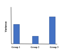
In statistics, Levene's test is an inferential statistic used to assess the equality of variances for a variable calculated for two or more groups. This test is used because some common statistical procedures assume that variances of the populations from which different samples are drawn are equal. Levene's test assesses this assumption. It tests the null hypothesis that the population variances are equal. If the resulting p-value of Levene's test is less than some significance level (typically 0.05), the obtained differences in sample variances are unlikely to have occurred based on random sampling from a population with equal variances. Thus, the null hypothesis of equal variances is rejected and it is concluded that there is a difference between the variances in the population.
Omnibus tests are a kind of statistical test. They test whether the explained variance in a set of data is significantly greater than the unexplained variance, overall. One example is the F-test in the analysis of variance. There can be legitimate significant effects within a model even if the omnibus test is not significant. For instance, in a model with two independent variables, if only one variable exerts a significant effect on the dependent variable and the other does not, then the omnibus test may be non-significant. This fact does not affect the conclusions that may be drawn from the one significant variable. In order to test effects within an omnibus test, researchers often use contrasts.
In statistics, one-way analysis of variance is a technique to compare whether two or more samples' means are significantly different. This analysis of variance technique requires a numeric response variable "Y" and a single explanatory variable "X", hence "one-way".
Tukey's range test, also known as Tukey's test, Tukey method, Tukey's honest significance test, or Tukey's HSDtest, is a single-step multiple comparison procedure and statistical test. It can be used to correctly interpret the statistical significance of the difference between means that have been selected for comparison because of their extreme values.
Named after the Dutch mathematician Bartel Leendert van der Waerden, the Van der Waerden test is a statistical test that k population distribution functions are equal. The Van der Waerden test converts the ranks from a standard Kruskal-Wallis test to quantiles of the standard normal distribution. These are called normal scores and the test is computed from these normal scores.
Repeated measures design is a research design that involves multiple measures of the same variable taken on the same or matched subjects either under different conditions or over two or more time periods. For instance, repeated measurements are collected in a longitudinal study in which change over time is assessed.
Multivariate analysis of covariance (MANCOVA) is an extension of analysis of covariance (ANCOVA) methods to cover cases where there is more than one dependent variable and where the control of concomitant continuous independent variables – covariates – is required. The most prominent benefit of the MANCOVA design over the simple MANOVA is the 'factoring out' of noise or error that has been introduced by the covariant. A commonly used multivariate version of the ANOVA F-statistic is Wilks' Lambda (Λ), which represents the ratio between the error variance and the effect variance.
In statistics, a mixed-design analysis of variance model, also known as a split-plot ANOVA, is used to test for differences between two or more independent groups whilst subjecting participants to repeated measures. Thus, in a mixed-design ANOVA model, one factor is a between-subjects variable and the other is a within-subjects variable. Thus, overall, the model is a type of mixed-effects model.
Exact statistics, such as that described in exact test, is a branch of statistics that was developed to provide more accurate results pertaining to statistical testing and interval estimation by eliminating procedures based on asymptotic and approximate statistical methods. The main characteristic of exact methods is that statistical tests and confidence intervals are based on exact probability statements that are valid for any sample size. Exact statistical methods help avoid some of the unreasonable assumptions of traditional statistical methods, such as the assumption of equal variances in classical ANOVA. They also allow exact inference on variance components of mixed models.
In statistics, one purpose for the analysis of variance (ANOVA) is to analyze differences in means between groups. The test statistic, F, assumes independence of observations, homogeneous variances, and population normality. ANOVA on ranks is a statistic designed for situations when the normality assumption has been violated.
In statistics, the two-way analysis of variance (ANOVA) is an extension of the one-way ANOVA that examines the influence of two different categorical independent variables on one continuous dependent variable. The two-way ANOVA not only aims at assessing the main effect of each independent variable but also if there is any interaction between them.
The Greenhouse–Geisser correction is a statistical method of adjusting for lack of sphericity in a repeated measures ANOVA. The correction functions as both an estimate of epsilon (sphericity) and a correction for lack of sphericity. The correction was proposed by Samuel Greenhouse and Seymour Geisser in 1959.
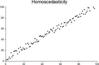
In statistics, a sequence of random variables is homoscedastic if all its random variables have the same finite variance; this is also known as homogeneity of variance. The complementary notion is called heteroscedasticity, also known as heterogeneity of variance. The spellings homoskedasticity and heteroskedasticity are also frequently used. “Skedasticity” comes from the Ancient Greek word “skedánnymi”, meaning “to scatter”. Assuming a variable is homoscedastic when in reality it is heteroscedastic results in unbiased but inefficient point estimates and in biased estimates of standard errors, and may result in overestimating the goodness of fit as measured by the Pearson coefficient.