Active contour model

Last updated

Active contour model, also called snakes, is a framework in computer vision introduced by Michael Kass, Andrew Witkin, and Demetri Terzopoulos [1] for delineating an object outline from a possibly noisy 2D image. The snakes model is popular in computer vision, and snakes are widely used in applications like object tracking, shape recognition, segmentation, edge detection and stereo matching.

Contents

A snake is an energy minimizing, deformable spline influenced by constraint and image forces that pull it towards object contours and internal forces that resist deformation. Snakes may be understood as a special case of the general technique of matching a deformable model to an image by means of energy minimization. [1] In two dimensions, the active shape model represents a discrete version of this approach, taking advantage of the point distribution model to restrict the shape range to an explicit domain learnt from a training set.

Snakes - active deformable models Snake-contour-example.jpg
Snakes – active deformable models

Snakes do not solve the entire problem of finding contours in images, since the method requires knowledge of the desired contour shape beforehand. Rather, they depend on other mechanisms such as interaction with a user, interaction with some higher level image understanding process, or information from image data adjacent in time or space.

Motivation

In computer vision, contour models describe the boundaries of shapes in an image. Snakes in particular are designed to solve problems where the approximate shape of the boundary is known. By being a deformable model, snakes can adapt to differences and noise in stereo matching and motion tracking. Additionally, the method can find Illusory contours in the image by ignoring missing boundary information.

Compared to classical feature extraction techniques, snakes have multiple advantages:

The key drawbacks of the traditional snakes are

Energy formulation

A simple elastic snake is defined by a set of n points for , the internal elastic energy term , and the external edge-based energy term . The purpose of the internal energy term is to control the deformations made to the snake, and the purpose of the external energy term is to control the fitting of the contour onto the image. The external energy is usually a combination of the forces due to the image itself and the constraint forces introduced by the user

The energy function of the snake is the sum of its external energy and internal energy, or

Internal energy

The internal energy of the snake is composed of the continuity of the contour and the smoothness of the contour .

[3]

This can be expanded as

where and are user-defined weights; these control the internal energy function's sensitivity to the amount of stretch in the snake and the amount of curvature in the snake, respectively, and thereby control the number of constraints on the shape of the snake.

In practice, a large weight for the continuity term penalizes changes in distances between points in the contour. A large weight for the smoothness term penalizes oscillations in the contour and will cause the contour to act as a thin plate.

Image energy

Energy in the image is some function of the features of the image. This is one of the most common points of modification in derivative methods. Features in images and images themselves can be processed in many and various ways.

For an image , lines, edges, and terminations present in the image, the general formulation of energy due to the image is

where , , are weights of these salient features. Higher weights indicate that the salient feature will have a larger contribution to the image force.

Line functional

The line functional is the intensity of the image, which can be represented as

The sign of will determine whether the line will be attracted to either dark lines or light lines.

Some smoothing or noise reduction may be used on the image, which then the line functional appears as

Edge functional

The edge functional is based on the image gradient. One implementation of this is

A snake originating far from the desired object contour may erroneously converge to some local minimum. Scale space continuation can be used in order to avoid these local minima. This is achieved by using a blur filter on the image and reducing the amount of blur as the calculation progresses to refine the fit of the snake. The energy functional using scale space continuation is

where is a Gaussian with standard deviation . Minima of this function fall on the zero-crossings of which define edges as per Marr–Hildreth theory.

Termination functional

Curvature of level lines in a slightly smoothed image can be used to detect corners and terminations in an image. Using this method, let be the image smoothed by

with gradient angle

unit vectors along the gradient direction

and unit vectors perpendicular to the gradient direction

The termination functional of energy can be represented as

Constraint energy

Some systems, including the original snakes implementation, allowed for user interaction to guide the snakes, not only in initial placement but also in their energy terms. Such constraint energy can be used to interactively guide the snakes towards or away from particular features.

Optimization through gradient descent

Given an initial guess for a snake, the energy function of the snake is iteratively minimized. Gradient descent minimization is one of the simplest optimizations which can be used to minimize snake energy. [4] Each iteration takes one step in the negative gradient of the point with controlled step size to find local minima. This gradient-descent minimization can be implemented as

Where is the force on the snake, which is defined by the negative of the gradient of the energy field.

Assuming the weights and are constant with respect to , this iterative method can be simplified to

Discrete approximation

In practice, images have finite resolution and can only be integrated over finite time steps . As such, discrete approximations must be made for practical implementation of snakes.

The energy function of the snake can be approximated by using the discrete points on the snake.

Consequentially, the forces of the snake can be approximated as

Gradient approximation can be done through any finite approximation method with respect to s, such as Finite difference.

Numerical instability due to discrete time

The introduction of discrete time into the algorithm can introduce updates which the snake is moved past the minima it is attracted to; this further can cause oscillations around the minima or lead to a different minima being found.

This can be avoided through tuning the time step such that the step size is never greater than a pixel due to the image forces. However, in regions of low energy, the internal energies will dominate the update.

Alternatively, the image forces can be normalized for each step such that the image forces only update the snake by one pixel. This can be formulated as

where is near the value of the pixel size. This avoids the problem of dominating internal energies that arise from tuning the time step. [5]

Numerical instability due to discrete space

The energies in a continuous image may have zero-crossing that do not exist as a pixel in the image. In this case, a point in the snake would oscillate between the two pixels that neighbor this zero-crossing. This oscillation can be avoided by using interpolation between pixels instead of nearest neighbor. [5]

Some variants of snakes

The default method of snakes has various limitation and corner cases where the convergence performs poorly. Several alternatives exist which addresses issues of the default method, though with their own trade-offs. A few are listed here.

GVF snake model

The gradient vector flow (GVF) snake model [6] addresses two issues with snakes:

In 2D, the GVF vector field minimizes the energy functional

where is a controllable smoothing term. This can be solved by solving the Euler equations

This can be solved through iteration towards a steady-state value.

This result replaces the default external force.

The primary issue with using GVF is the smoothing term causes rounding of the edges of the contour. Reducing the value of reduces the rounding but weakens the amount of smoothing.

The balloon model

The balloon model [5] addresses these problems with the default active contour model:

The balloon model introduces an inflation term into the forces acting on the snake

where is the normal unitary vector of the curve at and is the magnitude of the force. should have the same magnitude as the image normalization factor and be smaller in value than to allow forces at image edges to overcome the inflation force.

Three issues arise from using the balloon model:

Diffusion snakes model

The diffusion snake model [7] addresses the sensitivity of snakes to noise, clutter, and occlusion. It implements a modification of the Mumford–Shah functional and its cartoon limit and incorporates statistical shape knowledge. The default image energy functional is replaced with

where is based on a modified Mumford–Shah functional

where is the piecewise smooth model of the image of domain . Boundaries are defined as

where are quadratic B-spline basis functions and are the control points of the splines. The modified cartoon limit is obtained as and is a valid configuration of .

The functional is based on training from binary images of various contours and is controlled in strength by the parameter . For a Gaussian distribution of control point vectors with mean control point vector and covariance matrix , the quadratic energy that corresponds to the Gaussian probability is

The strength of this method relies on the strength of the training data as well as the tuning of the modified Mumford–Shah functional. Different snakes will require different training data sets and tunings.

Geometric active contours

Geometric active contour, or geodesic active contour (GAC) [8] or conformal active contours [9] employs ideas from Euclidean curve shortening evolution. Contours split and merge depending on the detection of objects in the image. These models are largely inspired by level sets, and have been extensively employed in medical image computing.

For example, the gradient descent curve evolution equation of GAC is [8]

where is a halting function, c is a Lagrange multiplier, is the curvature, and is the unit inward normal. This particular form of curve evolution equation is only dependent on the velocity in the normal direction. It therefore can be rewritten equivalently in an Eulerian form by inserting the level set function into it as follows

This simple yet powerful level-set reformation enables active contours to handle topology changes during the gradient descent curve evolution. It has inspired tremendous progress in the related fields, and using numerical methods to solve the level-set reformulation is now commonly known as the level-set method. Although the level set method has become quite a popular tool for implementing active contours, Wang and Chan argued that not all curve evolution equations should be directly solved by it. [10]

More recent developments in active contours address modeling of regional properties, incorporation of flexible shape priors and fully automatic segmentation, etc.

Statistical models combining local and global features have been formulated by Lankton and Allen Tannenbaum. [11]

Relations to graph cuts

Graph cuts, or max-flow/min-cut, is a generic method for minimizing a particular form of energy called Markov random field (MRF) energy. The Graph cuts method has been applied to image segmentation as well, and it sometimes outperforms the level set method when the model is MRF or can be approximated by MRF.

See also

Related Research Articles

<span class="mw-page-title-main">Generalized Stokes theorem</span> Statement about integration on manifolds

In vector calculus and differential geometry the generalized Stokes theorem, also called the Stokes–Cartan theorem, is a statement about the integration of differential forms on manifolds, which both simplifies and generalizes several theorems from vector calculus. In particular, the fundamental theorem of calculus is the special case where the manifold is a line segment, Green’s theorem and Stokes' theorem are the cases of a surface in or and the divergence theorem is the case of a volume in Hence, the theorem is sometimes referred to as the Fundamental Theorem of Multivariate Calculus.

<span class="mw-page-title-main">Potential flow</span> Velocity field as the gradient of a scalar function

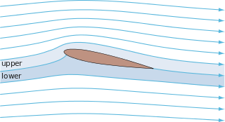
In fluid dynamics, potential flow describes the velocity field as the gradient of a scalar function: the velocity potential. As a result, a potential flow is characterized by an irrotational velocity field, which is a valid approximation for several applications. The irrotationality of a potential flow is due to the curl of the gradient of a scalar always being equal to zero.

Del, or nabla, is an operator used in mathematics as a vector differential operator, usually represented by the nabla symbol . When applied to a function defined on a one-dimensional domain, it denotes the standard derivative of the function as defined in calculus. When applied to a field, it may denote any one of three operations depending on the way it is applied: the gradient or (locally) steepest slope of a scalar field ; the divergence of a vector field; or the curl (rotation) of a vector field.

In mathematical optimization, the method of Lagrange multipliers is a strategy for finding the local maxima and minima of a function subject to equation constraints. It is named after the mathematician Joseph-Louis Lagrange. The basic idea is to convert a constrained problem into a form such that the derivative test of an unconstrained problem can still be applied. The relationship between the gradient of the function and gradients of the constraints rather naturally leads to a reformulation of the original problem, known as the Lagrangian function.

<span class="mw-page-title-main">Calculus of variations</span> Differential calculus on function spaces

The calculus of variations is a field of mathematical analysis that uses variations, which are small changes in functions and functionals, to find maxima and minima of functionals: mappings from a set of functions to the real numbers. Functionals are often expressed as definite integrals involving functions and their derivatives. Functions that maximize or minimize functionals may be found using the Euler–Lagrange equation of the calculus of variations.

<span class="mw-page-title-main">Green's function</span> Impulse response of an inhomogeneous linear differential operator

In mathematics, a Green's function is the impulse response of an inhomogeneous linear differential operator defined on a domain with specified initial conditions or boundary conditions.

A continuity equation or transport equation is an equation that describes the transport of some quantity. It is particularly simple and powerful when applied to a conserved quantity, but it can be generalized to apply to any extensive quantity. Since mass, energy, momentum, electric charge and other natural quantities are conserved under their respective appropriate conditions, a variety of physical phenomena may be described using continuity equations.

In mathematics, the covariant derivative is a way of specifying a derivative along tangent vectors of a manifold. Alternatively, the covariant derivative is a way of introducing and working with a connection on a manifold by means of a differential operator, to be contrasted with the approach given by a principal connection on the frame bundle – see affine connection. In the special case of a manifold isometrically embedded into a higher-dimensional Euclidean space, the covariant derivative can be viewed as the orthogonal projection of the Euclidean directional derivative onto the manifold's tangent space. In this case the Euclidean derivative is broken into two parts, the extrinsic normal component and the intrinsic covariant derivative component.

<span class="mw-page-title-main">Tensor calculus</span> Extension of vector calculus to tensors

In mathematics, tensor calculus, tensor analysis, or Ricci calculus is an extension of vector calculus to tensor fields.

In mathematics, the mean curvature of a surface is an extrinsic measure of curvature that comes from differential geometry and that locally describes the curvature of an embedded surface in some ambient space such as Euclidean space.

<span class="mw-page-title-main">Propagator</span> Function in quantum field theory showing probability amplitudes of moving particles

In quantum mechanics and quantum field theory, the propagator is a function that specifies the probability amplitude for a particle to travel from one place to another in a given period of time, or to travel with a certain energy and momentum. In Feynman diagrams, which serve to calculate the rate of collisions in quantum field theory, virtual particles contribute their propagator to the rate of the scattering event described by the respective diagram. These may also be viewed as the inverse of the wave operator appropriate to the particle, and are, therefore, often called (causal) Green's functions.

Geometrical optics, or ray optics, is a model of optics that describes light propagation in terms of rays. The ray in geometrical optics is an abstraction useful for approximating the paths along which light propagates under certain circumstances.

<span class="mw-page-title-main">Wave power</span> Transport of energy by wind waves, and the capture of that energy to do useful work

Wave power is the capture of energy of wind waves to do useful work – for example, electricity generation, water desalination, or pumping water. A machine that exploits wave power is a wave energy converter (WEC).

In differential geometry, the four-gradient is the four-vector analogue of the gradient from vector calculus.

When studying and formulating Albert Einstein's theory of general relativity, various mathematical structures and techniques are utilized. The main tools used in this geometrical theory of gravitation are tensor fields defined on a Lorentzian manifold representing spacetime. This article is a general description of the mathematics of general relativity.

<span class="mw-page-title-main">Lattice Boltzmann methods</span> Class of computational fluid dynamics methods

The lattice Boltzmann methods (LBM), originated from the lattice gas automata (LGA) method (Hardy-Pomeau-Pazzis and Frisch-Hasslacher-Pomeau models), is a class of computational fluid dynamics (CFD) methods for fluid simulation. Instead of solving the Navier–Stokes equations directly, a fluid density on a lattice is simulated with streaming and collision (relaxation) processes. The method is versatile as the model fluid can straightforwardly be made to mimic common fluid behaviour like vapour/liquid coexistence, and so fluid systems such as liquid droplets can be simulated. Also, fluids in complex environments such as porous media can be straightforwardly simulated, whereas with complex boundaries other CFD methods can be hard to work with.

<span class="mw-page-title-main">Spinodal decomposition</span> Mechanism of spontaneous phase separation

Spinodal decomposition is a mechanism by which a single thermodynamic phase spontaneously separates into two phases. Decomposition occurs when there is no thermodynamic barrier to phase separation. As a result, phase separation via decomposition does not require the nucleation events resulting from thermodynamic fluctuations, which normally trigger phase separation.

The Cauchy momentum equation is a vector partial differential equation put forth by Cauchy that describes the non-relativistic momentum transport in any continuum.

In fluid dynamics, the Oseen equations describe the flow of a viscous and incompressible fluid at small Reynolds numbers, as formulated by Carl Wilhelm Oseen in 1910. Oseen flow is an improved description of these flows, as compared to Stokes flow, with the (partial) inclusion of convective acceleration.

<span class="mw-page-title-main">Gradient vector flow</span>

Gradient vector flow (GVF), a computer vision framework introduced by Chenyang Xu and Jerry L. Prince, is the vector field that is produced by a process that smooths and diffuses an input vector field. It is usually used to create a vector field from images that points to object edges from a distance. It is widely used in image analysis and computer vision applications for object tracking, shape recognition, segmentation, and edge detection. In particular, it is commonly used in conjunction with active contour model.

References

  1. 1 2 Kass, M.; Witkin, A.; Terzopoulos, D. (1988). "Snakes: Active contour models" (PDF). International Journal of Computer Vision. 1 (4): 321. CiteSeerX   10.1.1.124.5318 . doi:10.1007/BF00133570. S2CID   12849354. Archived from the original (PDF) on 2016-01-12. Retrieved 2015-08-29.
  2. Snakes: an active model, Ramani Pichumani, http://homepages.inf.ed.ac.uk/rbf/CVonline/LOCAL_COPIES/RAMANI1/node31.html
  3. Dr. George Bebis, University of Nevada, http://www.cse.unr.edu/~bebis/CS791E/Notes/DeformableContours.pdf
  4. Image Understanding, Bryan S. Morse, Brigham Young University, 1998–2000 http://homepages.inf.ed.ac.uk/rbf/CVonline/LOCAL_COPIES/MORSE/iu.pdf
  5. 1 2 3 Cohen, Laurent D. (1991). "On active contour models and balloons". CVGIP: Image Understanding. 53 (2): 211–218. doi:10.1016/1049-9660(91)90028-N.
  6. Chenyang Xu; Prince, J.L. (1997). "Gradient vector flow: A new external force for snakes". Proceedings of IEEE Computer Society Conference on Computer Vision and Pattern Recognition (PDF). pp. 66–71. doi:10.1109/CVPR.1997.609299. ISBN   0-8186-7822-4. S2CID   980797.
  7. Cremers, D.; Schnorr, C.; Weickert, J. (2001). "Diffusion-snakes: Combining statistical shape knowledge and image information in a variational framework". Proceedings IEEE Workshop on Variational and Level Set Methods in Computer Vision. Vol. 50. pp. 137–144. CiteSeerX   10.1.1.28.3639 . doi:10.1109/VLSM.2001.938892. ISBN   978-0-7695-1278-5. S2CID   14929019.
  8. 1 2 Geodesic Active Contours, V. Caselles, R. Kimmel, G. Sapiro http://citeseerx.ist.psu.edu/viewdoc/summary?doi=10.1.1.21.2196
  9. Kichenassamy, Satyanad; Kumar, Arun; Olver, Peter; Tannenbaum, Allen; Yezzi, Anthony (1996). "Conformal curvature flows: From phase transitions to active vision". Archive for Rational Mechanics and Analysis. 134 (3): 275–301. Bibcode:1996ArRMA.134..275K. doi:10.1007/BF00379537. S2CID   116487549.
  10. Wang, Junyan; Chan, Kap Luk (2014-07-08). "Active Contour with a Tangential Component". Journal of Mathematical Imaging and Vision. 51 (2): 229–247. arXiv: 1204.6458 . doi:10.1007/s10851-014-0519-y. ISSN   0924-9907. S2CID   13100077.
  11. Lankton, S.; Tannenbaum, A. (2008). "Localizing Region-Based Active Contours". IEEE Transactions on Image Processing. 17 (11): 2029–2039. Bibcode:2008ITIP...17.2029L. doi:10.1109/TIP.2008.2004611. PMC   2796112 . PMID   18854247.

Sample code