Adaptive filter

Last updated

An adaptive filter is a system with a linear filter that has a transfer function controlled by variable parameters and a means to adjust those parameters according to an optimization algorithm. Because of the complexity of the optimization algorithms, almost all adaptive filters are digital filters. Adaptive filters are required for some applications because some parameters of the desired processing operation (for instance, the locations of reflective surfaces in a reverberant space) are not known in advance or are changing. The closed loop adaptive filter uses feedback in the form of an error signal to refine its transfer function.

Contents

Generally speaking, the closed loop adaptive process involves the use of a cost function, which is a criterion for optimum performance of the filter, to feed an algorithm, which determines how to modify filter transfer function to minimize the cost on the next iteration. The most common cost function is the mean square of the error signal.

As the power of digital signal processors has increased, adaptive filters have become much more common and are now routinely used in devices such as mobile phones and other communication devices, camcorders and digital cameras, and medical monitoring equipment.

Example application

The recording of a heart beat (an ECG), may be corrupted by noise from the AC mains. The exact frequency of the power and its harmonics may vary from moment to moment.

One way to remove the noise is to filter the signal with a notch filter at the mains frequency and its vicinity, but this could excessively degrade the quality of the ECG since the heart beat would also likely have frequency components in the rejected range.

To circumvent this potential loss of information, an adaptive filter could be used. The adaptive filter would take input both from the patient and from the mains and would thus be able to track the actual frequency of the noise as it fluctuates and subtract the noise from the recording. Such an adaptive technique generally allows for a filter with a smaller rejection range, which means, in this case, that the quality of the output signal is more accurate for medical purposes. [1] [2]

Block diagram

The idea behind a closed loop adaptive filter is that a variable filter is adjusted until the error (the difference between the filter output and the desired signal) is minimized. The Least Mean Squares (LMS) filter and the Recursive Least Squares (RLS) filter are types of adaptive filter.

Adaptive Filter. k = sample number, x = reference input, X = set of recent values of x, d = desired input, W = set of filter coefficients, e = error output, f = filter impulse response, * = convolution, S = summation, upper box=linear filter, lower box=adaption algorithm Adaptive Filter General.png
Adaptive Filter. k = sample number, x = reference input, X = set of recent values of x, d = desired input, W = set of filter coefficients, ε = error output, f = filter impulse response, * = convolution, Σ = summation, upper box=linear filter, lower box=adaption algorithm
Adaptive Filter, compact representation. k = sample number, x = reference input, d = desired input, e = error output, f = filter impulse response, S = summation, box=linear filter and adaption algorithm. Adaptive Filter Compact.png
Adaptive Filter, compact representation. k = sample number, x = reference input, d = desired input, ε = error output, f = filter impulse response, Σ = summation, box=linear filter and adaption algorithm.

There are two input signals to the adaptive filter: and which are sometimes called the primary input and the reference input respectively. [3] The adaptation algorithm attempts to filter the reference input into a replica of the desired input by minimizing the residual signal, . When the adaptation is successful, the output of the filter is effectively an estimate of the desired signal.

which includes the desired signal plus undesired interference and
which includes the signals that are correlated to some of the undesired interference in .
k represents the discrete sample number.

The filter is controlled by a set of L+1 coefficients or weights.

represents the set or vector of weights, which control the filter at sample time k.
where refers to the 'th weight at k'th time.
represents the change in the weights that occurs as a result of adjustments computed at sample time k.
These changes will be applied after sample time k and before they are used at sample time k+1.

The output is usually but it could be or it could even be the filter coefficients. [4] (Widrow)

The input signals are defined as follows:

where:
g = the desired signal,
g' = a signal that is correlated with the desired signal g ,
u = an undesired signal that is added to g , but not correlated with g or g'
u' = a signal that is correlated with the undesired signal u, but not correlated with g or g',
v = an undesired signal (typically random noise) not correlated with g, g', u, u' or v',
v' = an undesired signal (typically random noise) not correlated with g, g', u, u' or v.

The output signals are defined as follows:

.
where:
= the output of the filter if the input was only g',
= the output of the filter if the input was only u',
= the output of the filter if the input was only v'.

Tapped delay line FIR filter

If the variable filter has a tapped delay line Finite Impulse Response (FIR) structure, then the impulse response is equal to the filter coefficients. The output of the filter is given by

where refers to the 'th weight at k'th time.

Ideal case

In the ideal case . All the undesired signals in are represented by . consists entirely of a signal correlated with the undesired signal in .

The output of the variable filter in the ideal case is

.

The error signal or cost function is the difference between and

. The desired signal gk passes through without being changed.

The error signal is minimized in the mean square sense when is minimized. In other words, is the best mean square estimate of . In the ideal case, and , and all that is left after the subtraction is which is the unchanged desired signal with all undesired signals removed.

Signal components in the reference input

In some situations, the reference input includes components of the desired signal. This means g' ≠ 0.

Perfect cancelation of the undesired interference is not possible in the case, but improvement of the signal to interference ratio is possible. The output will be

. The desired signal will be modified (usually decreased).

The output signal to interference ratio has a simple formula referred to as power inversion.

.
where
= output signal to interference ratio.
= reference signal to interference ratio.
= frequency in the z-domain.

This formula means that the output signal to interference ratio at a particular frequency is the reciprocal of the reference signal to interference ratio. [5]

Example: A fast food restaurant has a drive-up window. Before getting to the window, customers place their order by speaking into a microphone. The microphone also picks up noise from the engine and the environment. This microphone provides the primary signal. The signal power from the customer's voice and the noise power from the engine are equal. It is difficult for the employees in the restaurant to understand the customer. To reduce the amount of interference in the primary microphone, a second microphone is located where it is intended to pick up sounds from the engine. It also picks up the customer's voice. This microphone is the source of the reference signal. In this case, the engine noise is 50 times more powerful than the customer's voice. Once the canceler has converged, the primary signal to interference ratio will be improved from 1:1 to 50:1.

Adaptive Linear Combiner

Adaptive linear combiner showing the combiner and the adaption process. k = sample number, n=input variable index, x = reference inputs, d = desired input, W = set of filter coefficients, e = error output, S = summation, upper box=linear combiner, lower box=adaption algorithm. Adaptive Linear Combiner General.png
Adaptive linear combiner showing the combiner and the adaption process. k = sample number, n=input variable index, x = reference inputs, d = desired input, W = set of filter coefficients, ε = error output, Σ = summation, upper box=linear combiner, lower box=adaption algorithm.
Adaptive linear combiner, compact representation. k = sample number, n=input variable index, x = reference inputs, d = desired input, e = error output, S = summation. Adaptive Linear Combiner Compact.png
Adaptive linear combiner, compact representation. k = sample number, n=input variable index, x = reference inputs, d = desired input, ε = error output, Σ = summation.

The adaptive linear combiner (ALC) resembles the adaptive tapped delay line FIR filter except that there is no assumed relationship between the X values. If the X values were from the outputs of a tapped delay line, then the combination of tapped delay line and ALC would comprise an adaptive filter. However, the X values could be the values of an array of pixels. Or they could be the outputs of multiple tapped delay lines. The ALC finds use as an adaptive beam former for arrays of hydrophones or antennas.

where refers to the 'th weight at k'th time.

LMS algorithm

If the variable filter has a tapped delay line FIR structure, then the LMS update algorithm is especially simple. Typically, after each sample, the coefficients of the FIR filter are adjusted as follows: [6]

for
μ is called the convergence factor.

The LMS algorithm does not require that the X values have any particular relationship; therefore it can be used to adapt a linear combiner as well as an FIR filter. In this case the update formula is written as:

The effect of the LMS algorithm is at each time, k, to make a small change in each weight. The direction of the change is such that it would decrease the error if it had been applied at time k. The magnitude of the change in each weight depends on μ, the associated X value and the error at time k. The weights making the largest contribution to the output, , are changed the most. If the error is zero, then there should be no change in the weights. If the associated value of X is zero, then changing the weight makes no difference, so it is not changed.

Convergence

μ controls how fast and how well the algorithm converges to the optimum filter coefficients. If μ is too large, the algorithm will not converge. If μ is too small the algorithm converges slowly and may not be able to track changing conditions. If μ is large but not too large to prevent convergence, the algorithm reaches steady state rapidly but continuously overshoots the optimum weight vector. Sometimes, μ is made large at first for rapid convergence and then decreased to minimize overshoot.

Widrow and Stearns state in 1985 that they have no knowledge of a proof that the LMS algorithm will converge in all cases. [7]

However under certain assumptions about stationarity and independence it can be shown that the algorithm will converge if

where
= sum of all input power
is the RMS value of the 'th input

In the case of the tapped delay line filter, each input has the same RMS value because they are simply the same values delayed. In this case the total power is

where
is the RMS value of , the input stream. [7]

This leads to a normalized LMS algorithm:

in which case the convergence criteria becomes: .

Nonlinear Adaptive Filters

The goal of nonlinear filters is to overcome limitation of linear models. There are some commonly used approaches: Volterra LMS, Kernel adaptive filter, Spline Adaptive Filter [8] and Urysohn Adaptive Filter. [9] [10] Many authors [11] include also Neural networks into this list. The general idea behind Volterra LMS and Kernel LMS is to replace data samples by different nonlinear algebraic expressions. For Volterra LMS this expression is Volterra series. In Spline Adaptive Filter the model is a cascade of linear dynamic block and static non-linearity, which is approximated by splines. In Urysohn Adaptive Filter the linear terms in a model

are replaced by piecewise linear functions

which are identified from data samples.

Applications of adaptive filters

Filter implementations

See also

Related Research Articles

Signal-to-noise ratio is a measure used in science and engineering that compares the level of a desired signal to the level of background noise. SNR is defined as the ratio of signal power to noise power, often expressed in decibels. A ratio higher than 1:1 indicates more signal than noise.

Linear elasticity is a mathematical model of how solid objects deform and become internally stressed due to prescribed loading conditions. It is a simplification of the more general nonlinear theory of elasticity and a branch of continuum mechanics.

In control systems, sliding mode control (SMC) is a nonlinear control method that alters the dynamics of a nonlinear system by applying a discontinuous control signal that forces the system to "slide" along a cross-section of the system's normal behavior. The state-feedback control law is not a continuous function of time. Instead, it can switch from one continuous structure to another based on the current position in the state space. Hence, sliding mode control is a variable structure control method. The multiple control structures are designed so that trajectories always move toward an adjacent region with a different control structure, and so the ultimate trajectory will not exist entirely within one control structure. Instead, it will slide along the boundaries of the control structures. The motion of the system as it slides along these boundaries is called a sliding mode and the geometrical locus consisting of the boundaries is called the sliding (hyper)surface. In the context of modern control theory, any variable structure system, like a system under SMC, may be viewed as a special case of a hybrid dynamical system as the system both flows through a continuous state space but also moves through different discrete control modes.

<span class="mw-page-title-main">Array processing</span>

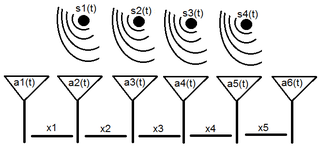
Array processing is a wide area of research in the field of signal processing that extends from the simplest form of 1 dimensional line arrays to 2 and 3 dimensional array geometries. Array structure can be defined as a set of sensors that are spatially separated, e.g. radio antenna and seismic arrays. The sensors used for a specific problem may vary widely, for example microphones, accelerometers and telescopes. However, many similarities exist, the most fundamental of which may be an assumption of wave propagation. Wave propagation means there is a systemic relationship between the signal received on spatially separated sensors. By creating a physical model of the wave propagation, or in machine learning applications a training data set, the relationships between the signals received on spatially separated sensors can be leveraged for many applications.

In statistics, econometrics, and signal processing, an autoregressive (AR) model is a representation of a type of random process; as such, it is used to describe certain time-varying processes in nature, economics, behavior, etc. The autoregressive model specifies that the output variable depends linearly on its own previous values and on a stochastic term ; thus the model is in the form of a stochastic difference equation. Together with the moving-average (MA) model, it is a special case and key component of the more general autoregressive–moving-average (ARMA) and autoregressive integrated moving average (ARIMA) models of time series, which have a more complicated stochastic structure; it is also a special case of the vector autoregressive model (VAR), which consists of a system of more than one interlocking stochastic difference equation in more than one evolving random variable.

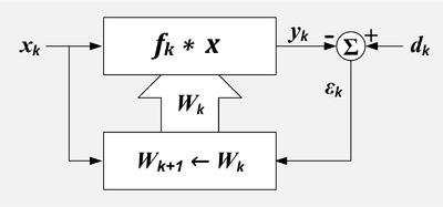
Least mean squares (LMS) algorithms are a class of adaptive filter used to mimic a desired filter by finding the filter coefficients that relate to producing the least mean square of the error signal. It is a stochastic gradient descent method in that the filter is only adapted based on the error at the current time. It was invented in 1960 by Stanford University professor Bernard Widrow and his first Ph.D. student, Ted Hoff.

Recursive least squares (RLS) is an adaptive filter algorithm that recursively finds the coefficients that minimize a weighted linear least squares cost function relating to the input signals. This approach is in contrast to other algorithms such as the least mean squares (LMS) that aim to reduce the mean square error. In the derivation of the RLS, the input signals are considered deterministic, while for the LMS and similar algorithms they are considered stochastic. Compared to most of its competitors, the RLS exhibits extremely fast convergence. However, this benefit comes at the cost of high computational complexity.

<span class="mw-page-title-main">ADALINE</span> Early single-layer artificial neural network

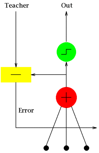
ADALINE is an early single-layer artificial neural network and the name of the physical device that implemented this network. The network uses memistors. It was developed by professor Bernard Widrow and his doctoral student Ted Hoff at Stanford University in 1960. It is based on the perceptron. It consists of a weight, a bias and a summation function.

The multidelay block frequency domain adaptive filter (MDF) algorithm is a block-based frequency domain implementation of the (normalised) Least mean squares filter (LMS) algorithm.

The Least mean squares filter solution converges to the Wiener filter solution, assuming that the unknown system is LTI and the noise is stationary. Both filters can be used to identify the impulse response of an unknown system, knowing only the original input signal and the output of the unknown system. By relaxing the error criterion to reduce current sample error instead of minimizing the total error over all of n, the LMS algorithm can be derived from the Wiener filter.

In the fields of computer vision and image analysis, the Harris affine region detector belongs to the category of feature detection. Feature detection is a preprocessing step of several algorithms that rely on identifying characteristic points or interest points so to make correspondences between images, recognize textures, categorize objects or build panoramas.

<span class="mw-page-title-main">Matrix completion</span>

Matrix completion is the task of filling in the missing entries of a partially observed matrix, which is equivalent to performing data imputation in statistics. A wide range of datasets are naturally organized in matrix form. One example is the movie-ratings matrix, as appears in the Netflix problem: Given a ratings matrix in which each entry represents the rating of movie by customer , if customer has watched movie and is otherwise missing, we would like to predict the remaining entries in order to make good recommendations to customers on what to watch next. Another example is the document-term matrix: The frequencies of words used in a collection of documents can be represented as a matrix, where each entry corresponds to the number of times the associated term appears in the indicated document.

A two-dimensional (2D) adaptive filter is very much like a one-dimensional adaptive filter in that it is a linear system whose parameters are adaptively updated throughout the process, according to some optimization approach. The main difference between 1D and 2D adaptive filters is that the former usually take as inputs signals with respect to time, what implies in causality constraints, while the latter handles signals with 2 dimensions, like x-y coordinates in the space domain, which are usually non-causal. Moreover, just like 1D filters, most 2D adaptive filters are digital filters, because of the complex and iterative nature of the algorithms.

The distributional learning theory or learning of probability distribution is a framework in computational learning theory. It has been proposed from Michael Kearns, Yishay Mansour, Dana Ron, Ronitt Rubinfeld, Robert Schapire and Linda Sellie in 1994 and it was inspired from the PAC-framework introduced by Leslie Valiant.

Carrier frequency offset (CFO) is one of many non-ideal conditions that may affect in baseband receiver design. In designing a baseband receiver, we should notice not only the degradation invoked by non-ideal channel and noise, we should also regard RF and analog parts as the main consideration. Those non-idealities include sampling clock offset, IQ imbalance, power amplifier, phase noise and carrier frequency offset nonlinearity.

<span class="mw-page-title-main">XPIC</span>

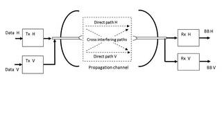
XPIC, or cross-polarization interference cancelling technology, is an algorithm to suppress mutual interference between two received streams in a Polarization-division multiplexing communication system.

<span class="mw-page-title-main">Batch normalization</span> Method used to make artificial neural networks faster and stable by re-centering and re-scaling

Batch normalization is a method used to make training of artificial neural networks faster and more stable through normalization of the layers' inputs by re-centering and re-scaling. It was proposed by Sergey Ioffe and Christian Szegedy in 2015.

Adding controlled noise from predetermined distributions is a way of designing differentially private mechanisms. This technique is useful for designing private mechanisms for real-valued functions on sensitive data. Some commonly used distributions for adding noise include Laplace and Gaussian distributions.

A guided filter is an edge-preserving smoothing image filter. As with a bilateral filter, it can filter out noise or texture while retaining sharp edges.

Adaptive noise cancelling is an unorthodox signal processing technique that is highly effective in suppressing additive interference or noise corrupting a received target signal at the main or primary sensor in certain common situations where the interference is known and is accessible but unavoidable and where the target signal and the interference are unrelated, that is, uncorrelated. Examples of such situations include:

References

  1. Thakor, N.V.; Zhu, Yi-Sheng (1991-08-01). "Applications of adaptive filtering to ECG analysis: noise cancellation and arrhythmia detection". IEEE Transactions on Biomedical Engineering. 38 (8): 785–794. doi:10.1109/10.83591. ISSN   0018-9294. PMID   1937512. S2CID   11271450.
  2. Widrow, Bernard; Stearns, Samuel D. (1985). Adaptive Signal Processing (1st ed.). Prentice-Hall. p.  329. ISBN   978-0130040299.
  3. Widrow p 304
  4. Widrow p 212
  5. Widrow p 313
  6. Widrow p. 100
  7. 1 2 Widrow p 103
  8. Danilo Comminiello; José C. Príncipe (2018). Adaptive Learning Methods for Nonlinear System Modeling. Elsevier Inc. ISBN   978-0-12-812976-0.
  9. M.Poluektov and A.Polar. Urysohn Adaptive Filter. 2019.
  10. "Nonlinear Adaptive Filtering". ezcodesample.com.
  11. Weifeng Liu; José C. Principe; Simon Haykin (March 2010). Kernel Adaptive Filtering: A Comprehensive Introduction (PDF). Wiley. pp. 12–20. ISBN   978-0-470-44753-6.

Sources