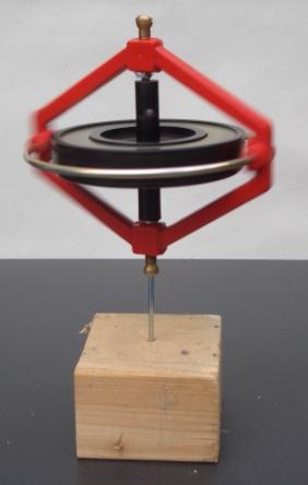
In physics, angular momentum is the rotational analog of linear momentum. It is an important physical quantity because it is a conserved quantity – the total angular momentum of a closed system remains constant. Angular momentum has both a direction and a magnitude, and both are conserved. Bicycles and motorcycles, flying discs, rifled bullets, and gyroscopes owe their useful properties to conservation of angular momentum. Conservation of angular momentum is also why hurricanes form spirals and neutron stars have high rotational rates. In general, conservation limits the possible motion of a system, but it does not uniquely determine it.

In relativity, proper time along a timelike world line is defined as the time as measured by a clock following that line. The proper time interval between two events on a world line is the change in proper time, which is independent of coordinates, and is a Lorentz scalar. The interval is the quantity of interest, since proper time itself is fixed only up to an arbitrary additive constant, namely the setting of the clock at some event along the world line.

In physics, the Rabi cycle is the cyclic behaviour of a two-level quantum system in the presence of an oscillatory driving field. A great variety of physical processes belonging to the areas of quantum computing, condensed matter, atomic and molecular physics, and nuclear and particle physics can be conveniently studied in terms of two-level quantum mechanical systems, and exhibit Rabi flopping when coupled to an optical driving field. The effect is important in quantum optics, magnetic resonance and quantum computing, and is named after Isidor Isaac Rabi.

In quantum mechanics, a two-state system is a quantum system that can exist in any quantum superposition of two independent quantum states. The Hilbert space describing such a system is two-dimensional. Therefore, a complete basis spanning the space will consist of two independent states. Any two-state system can also be seen as a qubit.

In physics, the Thomas precession, named after Llewellyn Thomas, is a relativistic correction that applies to the spin of an elementary particle or the rotation of a macroscopic gyroscope and relates the angular velocity of the spin of a particle following a curvilinear orbit to the angular velocity of the orbital motion.

In electromagnetism, the electromagnetic tensor or electromagnetic field tensor is a mathematical object that describes the electromagnetic field in spacetime. The field tensor was first used after the four-dimensional tensor formulation of special relativity was introduced by Hermann Minkowski. The tensor allows related physical laws to be written very concisely, and allows for the quantization of the electromagnetic field by Lagrangian formulation described below.
Self-phase modulation (SPM) is a nonlinear optical effect of light–matter interaction. An ultrashort pulse of light, when travelling in a medium, will induce a varying refractive index of the medium due to the optical Kerr effect. This variation in refractive index will produce a phase shift in the pulse, leading to a change of the pulse's frequency spectrum.
In MRI and NMR spectroscopy, an observable nuclear spin polarization (magnetization) is created by a homogeneous magnetic field. This field makes the magnetic dipole moments of the sample precess at the resonance (Larmor) frequency of the nuclei. At thermal equilibrium, nuclear spins precess randomly about the direction of the applied field. They become abruptly phase coherent when they are hit by radiofrequency (RF) pulses at the resonant frequency, created orthogonal to the field. The RF pulses cause the population of spin-states to be perturbed from their thermal equilibrium value. The generated transverse magnetization can then induce a signal in an RF coil that can be detected and amplified by an RF receiver. The return of the longitudinal component of the magnetization to its equilibrium value is termed spin-latticerelaxation while the loss of phase-coherence of the spins is termed spin-spin relaxation, which is manifest as an observed free induction decay (FID).
The covariant formulation of classical electromagnetism refers to ways of writing the laws of classical electromagnetism in a form that is manifestly invariant under Lorentz transformations, in the formalism of special relativity using rectilinear inertial coordinate systems. These expressions both make it simple to prove that the laws of classical electromagnetism take the same form in any inertial coordinate system, and also provide a way to translate the fields and forces from one frame to another. However, this is not as general as Maxwell's equations in curved spacetime or non-rectilinear coordinate systems.

In physics, the spin–spin relaxation is the mechanism by which Mxy, the transverse component of the magnetization vector, exponentially decays towards its equilibrium value in nuclear magnetic resonance (NMR) and magnetic resonance imaging (MRI). It is characterized by the spin–spin relaxation time, known as T2, a time constant characterizing the signal decay. It is named in contrast to T1, the spin–lattice relaxation time. It is the time it takes for the magnetic resonance signal to irreversibly decay to 37% (1/e) of its initial value after its generation by tipping the longitudinal magnetization towards the magnetic transverse plane. Hence the relation
The Weibel instability is a plasma instability present in homogeneous or nearly homogeneous electromagnetic plasmas which possess an anisotropy in momentum (velocity) space. This anisotropy is most generally understood as two temperatures in different directions. Burton Fried showed that this instability can be understood more simply as the superposition of many counter-streaming beams. In this sense, it is like the two-stream instability except that the perturbations are electromagnetic and result in filamentation as opposed to electrostatic perturbations which would result in charge bunching. In the linear limit the instability causes exponential growth of electromagnetic fields in the plasma which help restore momentum space isotropy. In very extreme cases, the Weibel instability is related to one- or two-dimensional stream instabilities.
An electric dipole transition is the dominant effect of an interaction of an electron in an atom with the electromagnetic field.
In continuum mechanics, a compatible deformation tensor field in a body is that unique tensor field that is obtained when the body is subjected to a continuous, single-valued, displacement field. Compatibility is the study of the conditions under which such a displacement field can be guaranteed. Compatibility conditions are particular cases of integrability conditions and were first derived for linear elasticity by Barré de Saint-Venant in 1864 and proved rigorously by Beltrami in 1886.
Rabi resonance method is a technique developed by Isidor Isaac Rabi for measuring the nuclear spin. The atom is placed in a static magnetic field and a perpendicular rotating magnetic field.
Pulsed electron paramagnetic resonance (EPR) is an electron paramagnetic resonance technique that involves the alignment of the net magnetization vector of the electron spins in a constant magnetic field. This alignment is perturbed by applying a short oscillating field, usually a microwave pulse. One can then measure the emitted microwave signal which is created by the sample magnetization. Fourier transformation of the microwave signal yields an EPR spectrum in the frequency domain. With a vast variety of pulse sequences it is possible to gain extensive knowledge on structural and dynamical properties of paramagnetic compounds. Pulsed EPR techniques such as electron spin echo envelope modulation (ESEEM) or pulsed electron nuclear double resonance (ENDOR) can reveal the interactions of the electron spin with its surrounding nuclear spins.

In the mathematics of dynamical systems, the double-scroll attractor is a strange attractor observed from a physical electronic chaotic circuit with a single nonlinear resistor. The double-scroll system is often described by a system of three nonlinear ordinary differential equations and a 3-segment piecewise-linear equation. This makes the system easily simulated numerically and easily manifested physically due to Chua's circuits' simple design.
Quantum stochastic calculus is a generalization of stochastic calculus to noncommuting variables. The tools provided by quantum stochastic calculus are of great use for modeling the random evolution of systems undergoing measurement, as in quantum trajectories. Just as the Lindblad master equation provides a quantum generalization to the Fokker–Planck equation, quantum stochastic calculus allows for the derivation of quantum stochastic differential equations (QSDE) that are analogous to classical Langevin equations.
Adiabatic radio frequency (RF) pulses are used in magnetic resonance imaging (MRI) to achieve excitation that is insensitive to spatial inhomogeneities in the excitation field or off-resonances in the sampled object.
In mathematics, differential forms on a Riemann surface are an important special case of the general theory of differential forms on smooth manifolds, distinguished by the fact that the conformal structure on the Riemann surface intrinsically defines a Hodge star operator on 1-forms without specifying a Riemannian metric. This allows the use of Hilbert space techniques for studying function theory on the Riemann surface and in particular for the construction of harmonic and holomorphic differentials with prescribed singularities. These methods were first used by Hilbert (1909) in his variational approach to the Dirichlet principle, making rigorous the arguments proposed by Riemann. Later Weyl (1940) found a direct approach using his method of orthogonal projection, a precursor of the modern theory of elliptic differential operators and Sobolev spaces. These techniques were originally applied to prove the uniformization theorem and its generalization to planar Riemann surfaces. Later they supplied the analytic foundations for the harmonic integrals of Hodge (1941). This article covers general results on differential forms on a Riemann surface that do not rely on any choice of Riemannian structure.
In mathematics, the exponential response formula (ERF), also known as exponential response and complex replacement, is a method used to find a particular solution of a non-homogeneous linear ordinary differential equation of any order. The exponential response formula is applicable to non-homogeneous linear ordinary differential equations with constant coefficients if the function is polynomial, sinusoidal, exponential or the combination of the three. The general solution of a non-homogeneous linear ordinary differential equation is a superposition of the general solution of the associated homogeneous ODE and a particular solution to the non-homogeneous ODE. Alternative methods for solving ordinary differential equations of higher order are method of undetermined coefficients and method of variation of parameters.


