
Independence is a fundamental notion in probability theory, as in statistics and the theory of stochastic processes. Two events are independent, statistically independent, or stochastically independent if, informally speaking, the occurrence of one does not affect the probability of occurrence of the other or, equivalently, does not affect the odds. Similarly, two random variables are independent if the realization of one does not affect the probability distribution of the other.

In probability theory, a probability density function (PDF), density function, or density of an absolutely continuous random variable, is a function whose value at any given sample in the sample space can be interpreted as providing a relative likelihood that the value of the random variable would be equal to that sample. Probability density is the probability per unit length, in other words, while the absolute likelihood for a continuous random variable to take on any particular value is 0, the value of the PDF at two different samples can be used to infer, in any particular draw of the random variable, how much more likely it is that the random variable would be close to one sample compared to the other sample.
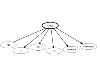
In statistics, naive Bayes classifiers are a family of simple "probabilistic classifiers" based on applying Bayes' theorem with strong (naive) independence assumptions between the features. They are among the simplest Bayesian network models, but coupled with kernel density estimation, they can achieve high accuracy levels.
In statistics, maximum likelihood estimation (MLE) is a method of estimating the parameters of an assumed probability distribution, given some observed data. This is achieved by maximizing a likelihood function so that, under the assumed statistical model, the observed data is most probable. The point in the parameter space that maximizes the likelihood function is called the maximum likelihood estimate. The logic of maximum likelihood is both intuitive and flexible, and as such the method has become a dominant means of statistical inference.
In mathematical optimization, the method of Lagrange multipliers is a strategy for finding the local maxima and minima of a function subject to equation constraints. It is named after the mathematician Joseph-Louis Lagrange.
In mathematical analysis, Hölder's inequality, named after Otto Hölder, is a fundamental inequality between integrals and an indispensable tool for the study of Lp spaces.
In mathematics, Fatou's lemma establishes an inequality relating the Lebesgue integral of the limit inferior of a sequence of functions to the limit inferior of integrals of these functions. The lemma is named after Pierre Fatou.

Given two random variables that are defined on the same probability space, the joint probability distribution is the corresponding probability distribution on all possible pairs of outputs. The joint distribution can just as well be considered for any given number of random variables. The joint distribution encodes the marginal distributions, i.e. the distributions of each of the individual random variables. It also encodes the conditional probability distributions, which deal with how the outputs of one random variable are distributed when given information on the outputs of the other random variable(s).

In probability and statistics, the Dirichlet distribution (after Peter Gustav Lejeune Dirichlet), often denoted , is a family of continuous multivariate probability distributions parameterized by a vector of positive reals. It is a multivariate generalization of the beta distribution, hence its alternative name of multivariate beta distribution (MBD). Dirichlet distributions are commonly used as prior distributions in Bayesian statistics, and in fact, the Dirichlet distribution is the conjugate prior of the categorical distribution and multinomial distribution.
In probability theory, if a large number of events are all independent of one another and each has probability less than 1, then there is a positive probability that none of the events will occur. The Lovász local lemma allows one to relax the independence condition slightly: As long as the events are "mostly" independent from one another and aren't individually too likely, then there will still be a positive probability that none of them occurs. It is most commonly used in the probabilistic method, in particular to give existence proofs.
In probability theory and statistics, the Dirichlet-multinomial distribution is a family of discrete multivariate probability distributions on a finite support of non-negative integers. It is also called the Dirichlet compound multinomial distribution (DCM) or multivariate Pólya distribution. It is a compound probability distribution, where a probability vector p is drawn from a Dirichlet distribution with parameter vector , and an observation drawn from a multinomial distribution with probability vector p and number of trials n. The Dirichlet parameter vector captures the prior belief about the situation and can be seen as a pseudocount: observations of each outcome that occur before the actual data is collected. The compounding corresponds to a Pólya urn scheme. It is frequently encountered in Bayesian statistics, machine learning, empirical Bayes methods and classical statistics as an overdispersed multinomial distribution.
In probability theory and theoretical computer science, McDiarmid's inequality is a concentration inequality which bounds the deviation between the sampled value and the expected value of certain functions when they are evaluated on independent random variables. McDiarmid's inequality applies to functions that satisfy a bounded differences property, meaning that replacing a single argument to the function while leaving all other arguments unchanged cannot cause too large of a change in the value of the function.
A continuous game is a mathematical concept, used in game theory, that generalizes the idea of an ordinary game like tic-tac-toe or checkers (draughts). In other words, it extends the notion of a discrete game, where the players choose from a finite set of pure strategies. The continuous game concepts allows games to include more general sets of pure strategies, which may be uncountably infinite.
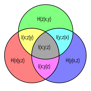
In probability theory, particularly information theory, the conditional mutual information is, in its most basic form, the expected value of the mutual information of two random variables given the value of a third.
Beliefs depend on the available information. This idea is formalized in probability theory by conditioning. Conditional probabilities, conditional expectations, and conditional probability distributions are treated on three levels: discrete probabilities, probability density functions, and measure theory. Conditioning leads to a non-random result if the condition is completely specified; otherwise, if the condition is left random, the result of conditioning is also random.
In probability theory, a Markov kernel is a map that in the general theory of Markov processes plays the role that the transition matrix does in the theory of Markov processes with a finite state space.
In probability theory, conditional probability is a measure of the probability of an event occurring, given that another event (by assumption, presumption, assertion or evidence) has already occurred. This particular method relies on event B occurring with some sort of relationship with another event A. In this event, the event B can be analyzed by a conditional probability with respect to A. If the event of interest is A and the event B is known or assumed to have occurred, "the conditional probability of A given B", or "the probability of A under the condition B", is usually written as P(A|B) or occasionally PB(A). This can also be understood as the fraction of probability B that intersects with A, or the ratio of the probabilities of both events happening to the "given" one happening (how many times A occurs rather than not assuming B has occurred): .
In statistics, a Pólya urn model, named after George Pólya, is a family of urn models that can be used to interpret many commonly used statistical models.
In machine learning, the kernel embedding of distributions comprises a class of nonparametric methods in which a probability distribution is represented as an element of a reproducing kernel Hilbert space (RKHS). A generalization of the individual data-point feature mapping done in classical kernel methods, the embedding of distributions into infinite-dimensional feature spaces can preserve all of the statistical features of arbitrary distributions, while allowing one to compare and manipulate distributions using Hilbert space operations such as inner products, distances, projections, linear transformations, and spectral analysis. This learning framework is very general and can be applied to distributions over any space on which a sensible kernel function may be defined. For example, various kernels have been proposed for learning from data which are: vectors in , discrete classes/categories, strings, graphs/networks, images, time series, manifolds, dynamical systems, and other structured objects. The theory behind kernel embeddings of distributions has been primarily developed by Alex Smola, Le Song , Arthur Gretton, and Bernhard Schölkopf. A review of recent works on kernel embedding of distributions can be found in.
In computational statistics, the pseudo-marginal Metropolis–Hastings algorithm is a Monte Carlo method to sample from a probability distribution. It is an instance of the popular Metropolis–Hastings algorithm that extends its use to cases where the target density is not available analytically. It relies on the fact that the Metropolis–Hastings algorithm can still sample from the correct target distribution if the target density in the acceptance ratio is replaced by an estimate. It is especially popular in Bayesian statistics, where it is applied if the likelihood function is not tractable.


