The Ising model, named after the physicists Ernst Ising and Wilhelm Lenz, is a mathematical model of ferromagnetism in statistical mechanics. The model consists of discrete variables that represent magnetic dipole moments of atomic "spins" that can be in one of two states. The spins are arranged in a graph, usually a lattice, allowing each spin to interact with its neighbors. Neighboring spins that agree have a lower energy than those that disagree; the system tends to the lowest energy but heat disturbs this tendency, thus creating the possibility of different structural phases. The model allows the identification of phase transitions as a simplified model of reality. The two-dimensional square-lattice Ising model is one of the simplest statistical models to show a phase transition.
In probability theory and mathematical physics, a random matrix is a matrix-valued random variable—that is, a matrix in which some or all elements are random variables. Many important properties of physical systems can be represented mathematically as matrix problems. For example, the thermal conductivity of a lattice can be computed from the dynamical matrix of the particle-particle interactions within the lattice.

The Hodgkin–Huxley model, or conductance-based model, is a mathematical model that describes how action potentials in neurons are initiated and propagated. It is a set of nonlinear differential equations that approximates the electrical engineering characteristics of excitable cells such as neurons and muscle cells. It is a continuous-time dynamical system.

The Lorenz system is a system of ordinary differential equations first studied by mathematician and meteorologist Edward Lorenz. It is notable for having chaotic solutions for certain parameter values and initial conditions. In particular, the Lorenz attractor is a set of chaotic solutions of the Lorenz system. In popular media the "butterfly effect" stems from the real-world implications of the Lorenz attractor, namely that several different initial chaotic conditions evolve in phase space in a way that never repeats, so all chaos is unpredictable. This underscores that chaotic systems can be completely deterministic and yet still be inherently unpredictable over long periods of time. Because chaos continually increases in systems, we cannot predict the future of systems well. E.g., even the small flap of a butterfly’s wings could set the world on a vastly different trajectory, such as by causing a hurricane. The shape of the Lorenz attractor itself, when plotted in phase space, may also be seen to resemble a butterfly.
In the field of mathematical modeling, a radial basis function network is an artificial neural network that uses radial basis functions as activation functions. The output of the network is a linear combination of radial basis functions of the inputs and neuron parameters. Radial basis function networks have many uses, including function approximation, time series prediction, classification, and system control. They were first formulated in a 1988 paper by Broomhead and Lowe, both researchers at the Royal Signals and Radar Establishment.
Synchronization of chaos is a phenomenon that may occur when two or more dissipative chaotic systems are coupled.
In computational neuroscience, the Wilson–Cowan model describes the dynamics of interactions between populations of very simple excitatory and inhibitory model neurons. It was developed by Hugh R. Wilson and Jack D. Cowan and extensions of the model have been widely used in modeling neuronal populations. The model is important historically because it uses phase plane methods and numerical solutions to describe the responses of neuronal populations to stimuli. Because the model neurons are simple, only elementary limit cycle behavior, i.e. neural oscillations, and stimulus-dependent evoked responses are predicted. The key findings include the existence of multiple stable states, and hysteresis, in the population response.

Biological neuron models, also known as a spiking neuron models, are mathematical descriptions of neurons. In particular, these models describe how the voltage potential across the cell membrane changes over time. In an experimental setting, stimulating neurons with an electrical current generates an action potential, that propagates down the neuron's axon. This axon can branch out and connect to a large number of downstream neurons at sites called synapses. At these synapses, the spike can cause release of a biochemical substance (neurotransmitter), which in turn can change the voltage potential of downstream neurons, potentially leading to spikes in those downstream neurons, thus propagating the signal. As many as 85% of neurons in the neocortex, the outermost layer of the mammalian brain, consists of excitatory pyramidal neurons, and each pyramidal neuron receives tens of thousands of inputs from other neurons. Thus, spiking neurons are a major information processing unit of the nervous system.
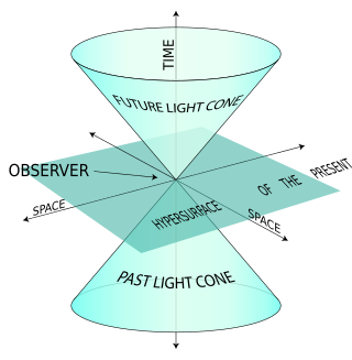
The light-front quantization of quantum field theories provides a useful alternative to ordinary equal-time quantization. In particular, it can lead to a relativistic description of bound systems in terms of quantum-mechanical wave functions. The quantization is based on the choice of light-front coordinates, where plays the role of time and the corresponding spatial coordinate is . Here, is the ordinary time, is one Cartesian coordinate, and is the speed of light. The other two Cartesian coordinates, and , are untouched and often called transverse or perpendicular, denoted by symbols of the type . The choice of the frame of reference where the time and -axis are defined can be left unspecified in an exactly soluble relativistic theory, but in practical calculations some choices may be more suitable than others.
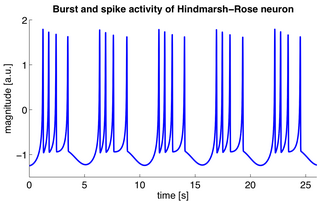
The Hindmarsh–Rose model of neuronal activity is aimed to study the spiking-bursting behavior of the membrane potential observed in experiments made with a single neuron. The relevant variable is the membrane potential, x(t), which is written in dimensionless units. There are two more variables, y(t) and z(t), which take into account the transport of ions across the membrane through the ion channels. The transport of sodium and potassium ions is made through fast ion channels and its rate is measured by y(t), which is called the spiking variable. z(t) corresponds to an adaptation current, which is incremented at every spike, leading to a decrease in the firing rate. Then, the Hindmarsh–Rose model has the mathematical form of a system of three nonlinear ordinary differential equations on the dimensionless dynamical variables x(t), y(t), and z(t). They read:
A coupled map lattice (CML) is a dynamical system that models the behavior of nonlinear systems. They are predominantly used to qualitatively study the chaotic dynamics of spatially extended systems. This includes the dynamics of spatiotemporal chaos where the number of effective degrees of freedom diverges as the size of the system increases.
The dynamical systems approach to neuroscience is a branch of mathematical biology that utilizes nonlinear dynamics to understand and model the nervous system and its functions. In a dynamical system, all possible states are expressed by a phase space. Such systems can experience bifurcation as a function of its bifurcation parameters and often exhibit chaos. Dynamical neuroscience describes the non-linear dynamics at many levels of the brain from single neural cells to cognitive processes, sleep states and the behavior of neurons in large-scale neuronal simulation.
Iterated filtering algorithms are a tool for maximum likelihood inference on partially observed dynamical systems. Stochastic perturbations to the unknown parameters are used to explore the parameter space. Applying sequential Monte Carlo to this extended model results in the selection of the parameter values that are more consistent with the data. Appropriately constructed procedures, iterating with successively diminished perturbations, converge to the maximum likelihood estimate. Iterated filtering methods have so far been used most extensively to study infectious disease transmission dynamics. Case studies include cholera, Ebola virus, influenza, malaria, HIV, pertussis, poliovirus and measles. Other areas which have been proposed to be suitable for these methods include ecological dynamics and finance.

The theta model, or Ermentrout–Kopell canonical model, is a biological neuron model originally developed to mathematically describe neurons in the animal Aplysia. The model is particularly well-suited to describe neural bursting, which is characterized by periodic transitions between rapid oscillations in the membrane potential followed by quiescence. This bursting behavior is often found in neurons responsible for controlling and maintaining steady rhythms such as breathing, swimming, and digesting. Of the three main classes of bursting neurons, the theta model describes parabolic bursting, which is characterized by a parabolic frequency curve during each burst.

The Rulkov map is a two-dimensional iterated map used to model a biological neuron. It was proposed by Nikolai F. Rulkov in 2001. The use of this map to study neural networks has computational advantages because the map is easier to iterate than a continuous dynamical system. This saves memory and simplifies the computation of large neural networks.
In the fields of dynamical systems and control theory, a fractional-order system is a dynamical system that can be modeled by a fractional differential equation containing derivatives of non-integer order. Such systems are said to have fractional dynamics. Derivatives and integrals of fractional orders are used to describe objects that can be characterized by power-law nonlocality, power-law long-range dependence or fractal properties. Fractional-order systems are useful in studying the anomalous behavior of dynamical systems in physics, electrochemistry, biology, viscoelasticity and chaotic systems.
The spike response model (SRM) is a spiking neuron model in which spikes are generated by either a deterministic or a stochastic threshold process. In the SRM, the membrane voltage V is described as a linear sum of the postsynaptic potentials (PSPs) caused by spike arrivals to which the effects of refractoriness and adaptation are added. The threshold is either fixed or dynamic. In the latter case it increases after each spike. The SRM is flexible enough to account for a variety of neuronal firing pattern in response to step current input. The SRM has also been used in the theory of computation to quantify the capacity of spiking neural networks; and in the neurosciences to predict the subthreshold voltage and the firing times of cortical neurons during stimulation with a time-dependent current stimulation. The name Spike Response Model points to the property that the two important filters and of the model can be interpreted as the response of the membrane potential to an incoming spike (response kernel , the PSP) and to an outgoing spike (response kernel , also called refractory kernel). The SRM has been formulated in continuous time and in discrete time. The SRM can be viewed as a generalized linear model (GLM) or as an (integrated version of) a generalized integrate-and-fire model with adaptation.
Tau functions are an important ingredient in the modern mathematical theory of integrable systems, and have numerous applications in a variety of other domains. They were originally introduced by Ryogo Hirota in his direct method approach to soliton equations, based on expressing them in an equivalent bilinear form.
In computational and mathematical biology, a biological lattice-gas cellular automaton (BIO-LGCA) is a discrete model for moving and interacting biological agents, a type of cellular automaton. The BIO-LGCA is based on the lattice-gas cellular automaton (LGCA) model used in fluid dynamics. A BIO-LGCA model describes cells and other motile biological agents as point particles moving on a discrete lattice, thereby interacting with nearby particles. Contrary to classic cellular automaton models, particles in BIO-LGCA are defined by their position and velocity. This allows to model and analyze active fluids and collective migration mediated primarily through changes in momentum, rather than density. BIO-LGCA applications include cancer invasion and cancer progression.

Synthetic Nervous System (SNS) is a computational neuroscience model that may be developed with the Functional Subnetwork Approach (FSA) to create biologically plausible models of circuits in a nervous system. The FSA enables the direct analytical tuning of dynamical networks that perform specific operations within the nervous system without the need for global optimization methods like genetic algorithms and reinforcement learning. The primary use case for a SNS is system control, where the system is most often a simulated biomechanical model or a physical robotic platform. An SNS is a form of a neural network much like artificial neural networks (ANNs), convolutional neural networks (CNN), and recurrent neural networks (RNN). The building blocks for each of these neural networks is a series of nodes and connections denoted as neurons and synapses. More conventional artificial neural networks rely on training phases where they use large data sets to form correlations and thus “learn” to identify a given object or pattern. When done properly this training results in systems that can produce a desired result, sometimes with impressive accuracy. However, the systems themselves are typically “black boxes” meaning there is no readily distinguishable mapping between structure and function of the network. This makes it difficult to alter the function, without simply starting over, or extract biological meaning except in specialized cases. The SNS method differentiates itself by using details of both structure and function of biological nervous systems. The neurons and synapse connections are intentionally designed rather than iteratively changed as part of a learning algorithm.


