
In mathematics, the discrete Fourier transform (DFT) converts a finite sequence of equally-spaced samples of a function into a same-length sequence of equally-spaced samples of the discrete-time Fourier transform (DTFT), which is a complex-valued function of frequency. The interval at which the DTFT is sampled is the reciprocal of the duration of the input sequence. An inverse DFT (IDFT) is a Fourier series, using the DTFT samples as coefficients of complex sinusoids at the corresponding DTFT frequencies. It has the same sample-values as the original input sequence. The DFT is therefore said to be a frequency domain representation of the original input sequence. If the original sequence spans all the non-zero values of a function, its DTFT is continuous, and the DFT provides discrete samples of one cycle. If the original sequence is one cycle of a periodic function, the DFT provides all the non-zero values of one DTFT cycle.
A fast Fourier transform (FFT) is an algorithm that computes the discrete Fourier transform (DFT) of a sequence, or its inverse (IDFT). Fourier analysis converts a signal from its original domain to a representation in the frequency domain and vice versa. The DFT is obtained by decomposing a sequence of values into components of different frequencies. This operation is useful in many fields, but computing it directly from the definition is often too slow to be practical. An FFT rapidly computes such transformations by factorizing the DFT matrix into a product of sparse factors. As a result, it manages to reduce the complexity of computing the DFT from , which arises if one simply applies the definition of DFT, to , where is the data size. The difference in speed can be enormous, especially for long data sets where N may be in the thousands or millions. In the presence of round-off error, many FFT algorithms are much more accurate than evaluating the DFT definition directly or indirectly. There are many different FFT algorithms based on a wide range of published theories, from simple complex-number arithmetic to group theory and number theory.
In mathematics, Fourier analysis is the study of the way general functions may be represented or approximated by sums of simpler trigonometric functions. Fourier analysis grew from the study of Fourier series, and is named after Joseph Fourier, who showed that representing a function as a sum of trigonometric functions greatly simplifies the study of heat transfer.
In mathematics, the convolution theorem states that under suitable conditions the Fourier transform of a convolution of two functions is the pointwise product of their Fourier transforms. More generally, convolution in one domain equals point-wise multiplication in the other domain. Other versions of the convolution theorem are applicable to various Fourier-related transforms.
A discrete cosine transform (DCT) expresses a finite sequence of data points in terms of a sum of cosine functions oscillating at different frequencies. The DCT, first proposed by Nasir Ahmed in 1972, is a widely used transformation technique in signal processing and data compression. It is used in most digital media, including digital images, digital video, digital audio, digital television, digital radio, and speech coding. DCTs are also important to numerous other applications in science and engineering, such as digital signal processing, telecommunication devices, reducing network bandwidth usage, and spectral methods for the numerical solution of partial differential equations.
In mathematics, the discrete sine transform (DST) is a Fourier-related transform similar to the discrete Fourier transform (DFT), but using a purely real matrix. It is equivalent to the imaginary parts of a DFT of roughly twice the length, operating on real data with odd symmetry (since the Fourier transform of a real and odd function is imaginary and odd), where in some variants the input and/or output data are shifted by half a sample.
A discrete Hartley transform (DHT) is a Fourier-related transform of discrete, periodic data similar to the discrete Fourier transform (DFT), with analogous applications in signal processing and related fields. Its main distinction from the DFT is that it transforms real inputs to real outputs, with no intrinsic involvement of complex numbers. Just as the DFT is the discrete analogue of the continuous Fourier transform (FT), the DHT is the discrete analogue of the continuous Hartley transform (HT), introduced by Ralph V. L. Hartley in 1942.
Rader's algorithm (1968), named for Charles M. Rader of MIT Lincoln Laboratory, is a fast Fourier transform (FFT) algorithm that computes the discrete Fourier transform (DFT) of prime sizes by re-expressing the DFT as a cyclic convolution.
Bruun's algorithm is a fast Fourier transform (FFT) algorithm based on an unusual recursive polynomial-factorization approach, proposed for powers of two by G. Bruun in 1978 and generalized to arbitrary even composite sizes by H. Murakami in 1996. Because its operations involve only real coefficients until the last computation stage, it was initially proposed as a way to efficiently compute the discrete Fourier transform (DFT) of real data. Bruun's algorithm has not seen widespread use, however, as approaches based on the ordinary Cooley–Tukey FFT algorithm have been successfully adapted to real data with at least as much efficiency. Furthermore, there is evidence that Bruun's algorithm may be intrinsically less accurate than Cooley–Tukey in the face of finite numerical precision.
The Cooley–Tukey algorithm, named after J. W. Cooley and John Tukey, is the most common fast Fourier transform (FFT) algorithm. It re-expresses the discrete Fourier transform (DFT) of an arbitrary composite size in terms of N1 smaller DFTs of sizes N2, recursively, to reduce the computation time to O(N log N) for highly composite N (smooth numbers). Because of the algorithm's importance, specific variants and implementation styles have become known by their own names, as described below.
In signal processing, a finite impulse response (FIR) filter is a filter whose impulse response is of finite duration, because it settles to zero in finite time. This is in contrast to infinite impulse response (IIR) filters, which may have internal feedback and may continue to respond indefinitely.
In mathematics, the discrete-time Fourier transform (DTFT), also called the finite Fourier transform, is a form of Fourier analysis that is applicable to a sequence of values.
The Goertzel algorithm is a technique in digital signal processing (DSP) for efficient evaluation of the individual terms of the discrete Fourier transform (DFT). It is useful in certain practical applications, such as recognition of dual-tone multi-frequency signaling (DTMF) tones produced by the push buttons of the keypad of a traditional analog telephone. The algorithm was first described by Gerald Goertzel in 1958.

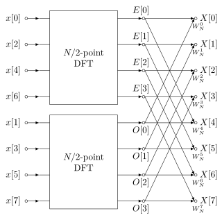
In the context of fast Fourier transform algorithms, a butterfly is a portion of the computation that combines the results of smaller discrete Fourier transforms (DFTs) into a larger DFT, or vice versa. The name "butterfly" comes from the shape of the data-flow diagram in the radix-2 case, as described below. The earliest occurrence in print of the term is thought to be in a 1969 MIT technical report. The same structure can also be found in the Viterbi algorithm, used for finding the most likely sequence of hidden states.
The split-radix FFT is a fast Fourier transform (FFT) algorithm for computing the discrete Fourier transform (DFT), and was first described in an initially little-appreciated paper by R. Yavne (1968) and subsequently rediscovered simultaneously by various authors in 1984. In particular, split radix is a variant of the Cooley–Tukey FFT algorithm that uses a blend of radices 2 and 4: it recursively expresses a DFT of length N in terms of one smaller DFT of length N/2 and two smaller DFTs of length N/4.

In signal processing, the overlap–add method is an efficient way to evaluate the discrete convolution of a very long signal with a finite impulse response (FIR) filter :
In mathematics, the discrete Fourier transform over a ring generalizes the discrete Fourier transform (DFT), of a function whose values are commonly complex numbers, over an arbitrary ring.

In signal processing, overlap–save is the traditional name for an efficient way to evaluate the discrete convolution between a very long signal and a finite impulse response (FIR) filter :
In mathematical analysis and applications, multidimensional transforms are used to analyze the frequency content of signals in a domain of two or more dimensions.
The fast Fourier transform (FFT) is an important tool in the fields of image and signal processing. The hexagonal fast Fourier transform (HFFT) uses existing FFT routines to compute the discrete Fourier transform (DFT) of images that have been captured with hexagonal sampling. The hexagonal grid serves as the optimal sampling lattice for isotropically band-limited two-dimensional signals and has a sampling efficiency which is 13.4% greater than the sampling efficiency obtained from rectangular sampling. Several other advantages of hexagonal sampling include consistent connectivity, higher symmetry, greater angular resolution, and equidistant neighbouring pixels. Sometimes, more than one of these advantages compound together, thereby increasing the efficiency by 50% in terms of computation and storage when compared to rectangular sampling. Despite all of these advantages of hexagonal sampling over rectangular sampling, its application has been limited because of the lack of an efficient coordinate system. However that limitation has been removed with the recent development of the hexagonal efficient coordinate system which includes the benefit of a separable Fourier kernel. The existence of a separable Fourier kernel for a hexagonally sampled image allows the use of existing FFT routines to efficiently compute the DFT of such an image.


