Constant-Q transform

Last updated

In mathematics and signal processing, the constant-Q transform and variable-Q transform, simply known as CQT and VQT, transforms a data series to the frequency domain. It is related to the Fourier transform [1] and very closely related to the complex Morlet wavelet transform. [2] Its design is suited for musical representation.

Contents

Constant-Q transform applied to the waveform of a C major piano chord. The x-axis is frequency, mapped to standard musical pitches, from low (left) to high (right). The y-axis is time, starting from pressing the piano chord at the bottom, and releasing the piano chord at the top, 8 seconds later. Darker pixels correspond to higher values of the Constant-Q transform. The peaks correspond closely to the precise frequencies of the vibrating piano strings. Thus the peaks can be used to detect the notes played on the piano. The lowest 3 peaks are the fundamental frequencies of the C major chord (C, E, G). Each string also vibrates at multiples of the fundamental, known as overtones, which correspond to the remaining smaller peaks to the right of the fundamental pitches. The overtones are smaller in intensity than the fundamental pitch.
Audio of the C Major piano chord used to generate the Constant-Q transform above.
Its waveform does not visually communicate pitch information like the Constant-Q transform is able to do. CQT-piano-chord.png
Constant-Q transform applied to the waveform of a C major piano chord. The x-axis is frequency, mapped to standard musical pitches, from low (left) to high (right). The y-axis is time, starting from pressing the piano chord at the bottom, and releasing the piano chord at the top, 8 seconds later. Darker pixels correspond to higher values of the Constant-Q transform. The peaks correspond closely to the precise frequencies of the vibrating piano strings. Thus the peaks can be used to detect the notes played on the piano. The lowest 3 peaks are the fundamental frequencies of the C major chord (C, E, G). Each string also vibrates at multiples of the fundamental, known as overtones, which correspond to the remaining smaller peaks to the right of the fundamental pitches. The overtones are smaller in intensity than the fundamental pitch.
Audio of the C Major piano chord used to generate the Constant-Q transform above.
Its waveform does not visually communicate pitch information like the Constant-Q transform is able to do. C-major-piano-chord-waveform.png
Its waveform does not visually communicate pitch information like the Constant-Q transform is able to do.

The transform can be thought of as a series of filters fk, logarithmically spaced in frequency, with the k-th filter having a spectral width δfk equal to a multiple of the previous filter's width:

where δfk is the bandwidth of the k-th filter, fmin is the central frequency of the lowest filter, and n is the number of filters per octave.

Calculation

The short-time Fourier transform of x[n] for a frame shifted to sample m is calculated as follows:

Given a data series at sampling frequency fs = 1/T, T being the sampling period of our data, for each frequency bin we can define the following:

This is shown below to be the integer number of cycles processed at a center frequency fk. As such, this somewhat defines the time complexity of the transform.
Since fs/fk is the number of samples processed per cycle at frequency fk, Q is the number of integer cycles processed at this central frequency.

The equivalent transform kernel can be found by using the following substitutions:

After these modifications, we are left with

Variable-Q bandwidth calculation

The variable-Q transform is the same as constant-Q transform, but the only difference is the filter Q is variable, hence the name variable-Q transform. The variable-Q transform is useful where time resolution on low frequencies is important[ examples needed ]. There are ways to calculate the bandwidth of the VQT, one of them using equivalent rectangular bandwidth as a value for VQT bin's bandwidth. [3]

The simplest way to implement a variable-Q transform is add a bandwidth offset called γ like this one:[ citation needed ]

This formula can be modified to have extra parameters to adjust sharpness of the transition between constant-Q and constant-bandwidth like this:[ citation needed ]

with α as a parameter for transition sharpness and where α of 2 is equals to hyperbolic sine frequency scale, in terms of frequency resolution.

Fast calculation

The direct calculation of the constant-Q transform (either using naive DFT or slightly faster Goertzel algorithm) is slow when compared against the fast Fourier transform (FFT). However, the FFT can itself be employed, in conjunction with the use of a kernel, to perform the equivalent calculation but much faster. [4] An approximate inverse to such an implementation was proposed in 2006; it works by going back to the DFT, and is only suitable for pitch instruments. [5]

A development on this method with improved invertibility involves performing CQT (via FFT) octave-by-octave, using lowpass filtered and downsampled results for consecutively lower pitches. [6] Implementations of this method include the MATLAB implementation and LibROSA's Python implementation. [7] LibROSA combines the subsampled method with the direct FFT method (which it dubs "pseudo-CQT") by having the latter process higher frequencies as a whole. [7]

The sliding DFT can be used for faster calculation of constant-Q transform, since the sliding DFT does not have to be linear-frequency spacing and same window size per bin. [8]

Alternatively, the constant-Q transform can be approximated by using multiple FFTs of different window sizes and/or sampling rate at different frequency ranges then stitch it together. This is called multiresolution STFT, however the window sizes for multiresolution FFTs are different per-octave, rather than per-bin.[ citation needed ][ ambiguous ]

Comparison with the Fourier transform

In general, the transform is well suited to musical data, and this can be seen in some of its advantages compared to the fast Fourier transform. As the output of the transform is effectively amplitude/phase against log frequency, fewer frequency bins are required to cover a given range effectively, and this proves useful where frequencies span several octaves. As the range of human hearing covers approximately ten octaves from 20 Hz to around 20 kHz, this reduction in output data is significant.

The transform exhibits a reduction in frequency resolution with higher frequency bins, which is desirable for auditory applications. The transform mirrors the human auditory system, whereby at lower-frequencies spectral resolution is better, whereas temporal resolution improves at higher frequencies. At the bottom of the piano scale (about 30 Hz), a difference of 1 semitone is a difference of approximately 1.5 Hz, whereas at the top of the musical scale (about 5 kHz), a difference of 1 semitone is a difference of approximately 200 Hz. [9] So for musical data the exponential frequency resolution of constant-Q transform is ideal.

In addition, the harmonics of musical notes form a pattern characteristic of the timbre of the instrument in this transform. Assuming the same relative strengths of each harmonic, as the fundamental frequency changes, the relative position of these harmonics remains constant. This can make identification of instruments much easier. The constant Q transform can also be used for automatic recognition of musical keys based on accumulated chroma content. [10]

Relative to the Fourier transform, implementation of this transform is more tricky. This is due to the varying number of samples used in the calculation of each frequency bin, which also affects the length of any windowing function implemented. [11]

Also note that because the frequency scale is logarithmic, there is no true zero-frequency / DC term present, which may be a drawback in applications that are interested in the DC term. Although for applications that are not interested in the DC such as audio, this is not a drawback.

Related Research Articles

<span class="mw-page-title-main">Discrete Fourier transform</span> Type of Fourier transform in discrete mathematics

In mathematics, the discrete Fourier transform (DFT) converts a finite sequence of equally-spaced samples of a function into a same-length sequence of equally-spaced samples of the discrete-time Fourier transform (DTFT), which is a complex-valued function of frequency. The interval at which the DTFT is sampled is the reciprocal of the duration of the input sequence. An inverse DFT (IDFT) is a Fourier series, using the DTFT samples as coefficients of complex sinusoids at the corresponding DTFT frequencies. It has the same sample-values as the original input sequence. The DFT is therefore said to be a frequency domain representation of the original input sequence. If the original sequence spans all the non-zero values of a function, its DTFT is continuous, and the DFT provides discrete samples of one cycle. If the original sequence is one cycle of a periodic function, the DFT provides all the non-zero values of one DTFT cycle.

<span class="mw-page-title-main">Fourier analysis</span> Branch of mathematics

In mathematics, Fourier analysis is the study of the way general functions may be represented or approximated by sums of simpler trigonometric functions. Fourier analysis grew from the study of Fourier series, and is named after Joseph Fourier, who showed that representing a function as a sum of trigonometric functions greatly simplifies the study of heat transfer.

<span class="mw-page-title-main">Wavelet</span> Function for integral Fourier-like transform

A wavelet is a wave-like oscillation with an amplitude that begins at zero, increases or decreases, and then returns to zero one or more times. Wavelets are termed a "brief oscillation". A taxonomy of wavelets has been established, based on the number and direction of its pulses. Wavelets are imbued with specific properties that make them useful for signal processing.

A low-pass filter is a filter that passes signals with a frequency lower than a selected cutoff frequency and attenuates signals with frequencies higher than the cutoff frequency. The exact frequency response of the filter depends on the filter design. The filter is sometimes called a high-cut filter, or treble-cut filter in audio applications. A low-pass filter is the complement of a high-pass filter.

<span class="mw-page-title-main">Morlet wavelet</span>

In mathematics, the Morlet wavelet is a wavelet composed of a complex exponential (carrier) multiplied by a Gaussian window (envelope). This wavelet is closely related to human perception, both hearing and vision.

<i>Q</i> factor Parameter describing the longevity of energy in a resonator relative to its resonant frequency

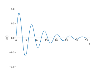
In physics and engineering, the quality factor or Q factor is a dimensionless parameter that describes how underdamped an oscillator or resonator is. It is defined as the ratio of the initial energy stored in the resonator to the energy lost in one radian of the cycle of oscillation. Q factor is alternatively defined as the ratio of a resonator's centre frequency to its bandwidth when subject to an oscillating driving force. These two definitions give numerically similar, but not identical, results. Higher Q indicates a lower rate of energy loss and the oscillations die out more slowly. A pendulum suspended from a high-quality bearing, oscillating in air, has a high Q, while a pendulum immersed in oil has a low one. Resonators with high quality factors have low damping, so that they ring or vibrate longer.

<span class="mw-page-title-main">Window function</span> Function used in signal processing

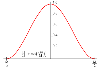
In signal processing and statistics, a window function is a mathematical function that is zero-valued outside of some chosen interval. Typically, windows functions are symmetric around the middle of the interval, approach a maximum in the middle, and taper away from the middle. Mathematically, when another function or waveform/data-sequence is "multiplied" by a window function, the product is also zero-valued outside the interval: all that is left is the part where they overlap, the "view through the window". Equivalently, and in actual practice, the segment of data within the window is first isolated, and then only that data is multiplied by the window function values. Thus, tapering, not segmentation, is the main purpose of window functions.

<span class="mw-page-title-main">Short-time Fourier transform</span> Fourier-related transform suited to signals that change rather quickly in time

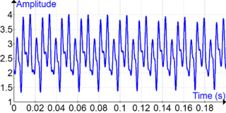
The short-time Fourier transform (STFT), is a Fourier-related transform used to determine the sinusoidal frequency and phase content of local sections of a signal as it changes over time. In practice, the procedure for computing STFTs is to divide a longer time signal into shorter segments of equal length and then compute the Fourier transform separately on each shorter segment. This reveals the Fourier spectrum on each shorter segment. One then usually plots the changing spectra as a function of time, known as a spectrogram or waterfall plot, such as commonly used in software defined radio (SDR) based spectrum displays. Full bandwidth displays covering the whole range of an SDR commonly use fast Fourier transforms (FFTs) with 2^24 points on desktop computers.

In signal processing, a finite impulse response (FIR) filter is a filter whose impulse response is of finite duration, because it settles to zero in finite time. This is in contrast to infinite impulse response (IIR) filters, which may have internal feedback and may continue to respond indefinitely.

The Fourier transform of a function of time, s(t), is a complex-valued function of frequency, S(f), often referred to as a frequency spectrum. Any linear time-invariant operation on s(t) produces a new spectrum of the form H(f)•S(f), which changes the relative magnitudes and/or angles (phase) of the non-zero values of S(f). Any other type of operation creates new frequency components that may be referred to as spectral leakage in the broadest sense. Sampling, for instance, produces leakage, which we call aliases of the original spectral component. For Fourier transform purposes, sampling is modeled as a product between s(t) and a Dirac comb function. The spectrum of a product is the convolution between S(f) and another function, which inevitably creates the new frequency components. But the term 'leakage' usually refers to the effect of windowing, which is the product of s(t) with a different kind of function, the window function. Window functions happen to have finite duration, but that is not necessary to create leakage. Multiplication by a time-variant function is sufficient.

<span class="mw-page-title-main">Discrete wavelet transform</span> Transform in numerical harmonic analysis

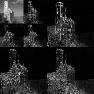
In numerical analysis and functional analysis, a discrete wavelet transform (DWT) is any wavelet transform for which the wavelets are discretely sampled. As with other wavelet transforms, a key advantage it has over Fourier transforms is temporal resolution: it captures both frequency and location information.

Stransform as a time–frequency distribution was developed in 1994 for analyzing geophysics data. In this way, the S transform is a generalization of the short-time Fourier transform (STFT), extending the continuous wavelet transform and overcoming some of its disadvantages. For one, modulation sinusoids are fixed with respect to the time axis; this localizes the scalable Gaussian window dilations and translations in S transform. Moreover, the S transform doesn't have a cross-term problem and yields a better signal clarity than Gabor transform. However, the S transform has its own disadvantages: the clarity is worse than Wigner distribution function and Cohen's class distribution function.

In mathematics, in the area of harmonic analysis, the fractional Fourier transform (FRFT) is a family of linear transformations generalizing the Fourier transform. It can be thought of as the Fourier transform to the n-th power, where n need not be an integer — thus, it can transform a function to any intermediate domain between time and frequency. Its applications range from filter design and signal analysis to phase retrieval and pattern recognition.

In mathematics, the discrete-time Fourier transform (DTFT) is a form of Fourier analysis that is applicable to a sequence of discrete values.

The Goertzel algorithm is a technique in digital signal processing (DSP) for efficient evaluation of the individual terms of the discrete Fourier transform (DFT). It is useful in certain practical applications, such as recognition of dual-tone multi-frequency signaling (DTMF) tones produced by the push buttons of the keypad of a traditional analog telephone. The algorithm was first described by Gerald Goertzel in 1958.

<span class="mw-page-title-main">Wavelet transform</span> Mathematical technique used in data compression and analysis

In mathematics, a wavelet series is a representation of a square-integrable function by a certain orthonormal series generated by a wavelet. This article provides a formal, mathematical definition of an orthonormal wavelet and of the integral wavelet transform.

In mathematics, Fourier–Bessel series is a particular kind of generalized Fourier series based on Bessel functions.

Fractional wavelet transform (FRWT) is a generalization of the classical wavelet transform (WT). This transform is proposed in order to rectify the limitations of the WT and the fractional Fourier transform (FRFT). The FRWT inherits the advantages of multiresolution analysis of the WT and has the capability of signal representations in the fractional domain which is similar to the FRFT.

In rotordynamics, order tracking is a family of signal processing tools aimed at transforming a measured signal from time domain to angular domain. These techniques are applied to asynchronously sampled signals to obtain the same signal sampled at constant angular increments of a reference shaft. In some cases the outcome of the Order Tracking is directly the Fourier transform of such angular domain signal, whose frequency counterpart is defined as "order". Each order represents a fraction of the angular velocity of the reference shaft.

The spectrum of a chirp pulse describes its characteristics in terms of its frequency components. This frequency-domain representation is an alternative to the more familiar time-domain waveform, and the two versions are mathematically related by the Fourier transform. The spectrum is of particular interest when pulses are subject to signal processing. For example, when a chirp pulse is compressed by its matched filter, the resulting waveform contains not only a main narrow pulse but, also, a variety of unwanted artifacts many of which are directly attributable to features in the chirp's spectral characteristics.

References

  1. Judith C. Brown, Calculation of a constant Q spectral transform, J. Acoust. Soc. Am., 89(1):425–434, 1991.
  2. Continuous Wavelet Transform "When the mother wavelet can be interpreted as a windowed sinusoid (such as the Morlet wavelet), the wavelet transform can be interpreted as a constant-Q Fourier transform. Before the theory of wavelets, constant-Q Fourier transforms (such as obtained from a classic third-octave filter bank) were not easy to invert, because the basis signals were not orthogonal."
  3. Cwitkowitz, Frank C.Jr (2019). "End-to-End Music Transcription Using Fine-Tuned Variable-Q Filterbanks" (PDF). Rochester Institute of Technology: 32–34. Retrieved 2022-08-21.
  4. Judith C. Brown and Miller S. Puckette, An efficient algorithm for the calculation of a constant Q transform, J. Acoust. Soc. Am., 92(5):2698–2701, 1992.
  5. FitzGerald, Derry; Cychowski, Marcin T.; Cranitch, Matt (1 May 2006). "Towards an Inverse Constant Q Transform". Audio Engineering Society Convention. Paris: Audio Engineering Society. 120.
  6. Schörkhuber, Christian; Klapuri, Anssi (2010). "CONSTANT-Q TRANSFORM TOOLBOX FOR MUSIC PROCESSING". 7th Sound and Music Computing Conference. Barcelona. Retrieved 12 December 2018. paper
  7. 1 2 McFee, Brian; Battenberg, Eric; Lostanlen, Vincent; Thomé, Carl (12 December 2018). "librosa: core/constantq.py at 8d26423". GitHub. librosa. Retrieved 12 December 2018.
  8. Bradford, R, ffitch, J & Dobson, R 2008, Sliding with a constant-Q, in 11th International Conference on Digital Audio Effects (DAFx-08) Proceedings September 1-4th, 2008 Espoo, Finland . DAFx, Espoo, Finland, pp. 363-369, Proc. of the Int. Conf. on Digital Audio Effects (DAFx-08), 1/09/08.
  9. http://newt.phys.unsw.edu.au/jw/graphics/notes.GIF [ bare URL image file ]
  10. Hendrik Purwins, Benjamin Blankertz and Klaus Obermayer, A New Method for Tracking Modulations in Tonal Music in Audio Data Format, International Joint Conference on Neural Network (IJCNN’00)., 6:270-275, 2000.
  11. Benjamin Blankertz, The Constant Q Transform, 1999.