Coordinate systems for the hyperbolic plane

Last updated

In the hyperbolic plane, as in the Euclidean plane, each point can be uniquely identified by two real numbers. Several qualitatively different ways of coordinatizing the plane in hyperbolic geometry are used.

Contents

This article tries to give an overview of several coordinate systems in use for the two-dimensional hyperbolic plane.

In the descriptions below the constant Gaussian curvature of the plane is −1. Sinh, cosh and tanh are hyperbolic functions.

Polar coordinate system

Points in the polar coordinate system with pole O and polar axis L. In green, the point with radial coordinate 3 and angular coordinate 60 degrees or (3, 60deg). In blue, the point (4, 210deg). Examples of Polar Coordinates.svg
Points in the polar coordinate system with pole O and polar axis L. In green, the point with radial coordinate 3 and angular coordinate 60 degrees or (3, 60°). In blue, the point (4, 210°).

The polar coordinate system is a two-dimensional coordinate system in which each point on a plane is determined by a distance from a reference point and an angle from a reference direction.

The reference point (analogous to the origin of a Cartesian system) is called the pole, and the ray from the pole in the reference direction is the polar axis. The distance from the pole is called the radial coordinate or radius, and the angle is called the angular coordinate, or polar angle.

From the hyperbolic law of cosines, we get that the distance between two points given in polar coordinates is

Let , differentiating at :

we get the corresponding metric tensor:

The straight lines are described by equations of the form

where r0 and θ0 are the coordinates of the nearest point on the line to the pole.

Quadrant model system

The Poincaré half-plane model is closely related to a model of the hyperbolic plane in the quadrant Q = {(x,y): x > 0, y > 0}. For such a point the geometric mean and the hyperbolic angle produce a point (u,v) in the upper half-plane. The hyperbolic metric in the quadrant depends on the Poincaré half-plane metric. The motions of the Poincaré model carry over to the quadrant; in particular the left or right shifts of the real axis correspond to hyperbolic rotations of the quadrant. Due to the study of ratios in physics and economics where the quadrant is the universe of discourse, its points are said to be located by hyperbolic coordinates.

Cartesian-style coordinate systems

In hyperbolic geometry rectangles do not exist. The sum of the angles of a quadrilateral in hyperbolic geometry is always less than 4 right angles (see Lambert quadrilateral). Also in hyperbolic geometry there are no equidistant lines (see hypercycles). This all has influences on the coordinate systems.

There are however different coordinate systems for hyperbolic plane geometry. All are based on choosing a real (non ideal) point (the Origin) on a chosen directed line (the x-axis) and after that many choices exist.

Axial coordinates

Axial coordinates xa and ya are found by constructing a y-axis perpendicular to the x-axis through the origin. [1]

Like in the Cartesian coordinate system, the coordinates are found by dropping perpendiculars from the point onto the x and y-axes. xa is the distance from the foot of the perpendicular on the x-axis to the origin (regarded as positive on one side and negative on the other); ya is the distance from the foot of the perpendicular on the y-axis to the origin.

Circles about the origin in hyperbolic axial coordinates. Circles about the origin in hyperbolic axial coordinates.gif
Circles about the origin in hyperbolic axial coordinates.

Every point and most ideal points have axial coordinates, but not every pair of real numbers corresponds to a point.

If then is an ideal point.

If then is not a point at all.

The distance of a point to the x-axis is . To the y-axis it is .

The relationship of axial coordinates to polar coordinates (assuming the origin is the pole and that the positive x-axis is the polar axis) is

Lobachevsky coordinates

The Lobachevsky coordinates x and y are found by dropping a perpendicular onto the x-axis. x is the distance from the foot of the perpendicular to the x-axis to the origin (positive on one side and negative on the other, the same as in axial coordinates). [1]

y is the distance along the perpendicular of the given point to its foot (positive on one side and negative on the other).

.

The Lobachevsky coordinates are useful for integration for length of curves [2] and area between lines and curves.[ example needed ]

Lobachevsky coordinates are named after Nikolai Lobachevsky one of the discoverers of hyperbolic geometry.

Circles about the origin of radius 1, 5 and 10 in the Lobachevsky hyperbolic coordinates. Circles in Lobachevsky hyperbolic coordinates.png
Circles about the origin of radius 1, 5 and 10 in the Lobachevsky hyperbolic coordinates.
Circles about the points (0,0), (0,1), (0,2) and (0,3) of radius 3.5 in the Lobachevsky hyperbolic coordinates. Circles of fixed radius in Lobachevsky hyperbolic coordinates.png
Circles about the points (0,0), (0,1), (0,2) and (0,3) of radius 3.5 in the Lobachevsky hyperbolic coordinates.

Construct a Cartesian-like coordinate system as follows. Choose a line (the x-axis) in the hyperbolic plane (with a standardized curvature of -1) and label the points on it by their distance from an origin (x=0) point on the x-axis (positive on one side and negative on the other). For any point in the plane, one can define coordinates x and y by dropping a perpendicular onto the x-axis. x will be the label of the foot of the perpendicular. y will be the distance along the perpendicular of the given point from its foot (positive on one side and negative on the other). Then the distance between two such points will be

This formula can be derived from the formulas about hyperbolic triangles.

The corresponding metric tensor is: .

In this coordinate system, straight lines are either perpendicular to the x-axis (with equation x = a constant) or described by equations of the form

where A and B are real parameters which characterize the straight line.

The relationship of Lobachevsky coordinates to polar coordinates (assuming the origin is the pole and that the positive x-axis is the polar axis) is

Horocycle-based coordinate system

Horocycle-based coordinate system Horocycle-based coordinate system.svg
Horocycle-based coordinate system

Another coordinate system uses the distance from the point to the horocycle through the origin centered around [ clarification needed ] and the arclength along this horocycle. [3]

Draw the horocycle hO through the origin centered at the ideal point at the end of the x-axis.

From point P draw the line p asymptotic to the x-axis to the right ideal point . Ph is the intersection of line p and horocycle hO.

The coordinate xh is the distance from P to Ph[ clarification needed ] – positive if P is between Ph and , negative if Ph is between P and .

The coordinate yh is the arclength along horocycle hO from the origin to Ph.[ clarification needed ]

The distance between two points given in these coordinates is

The corresponding metric tensor is:

The straight lines are described by equations of the form y = a constant or

where x0 and y0 are the coordinates of the point on the line nearest to the ideal point (i.e. having the largest value of x on the line).

Model-based coordinate systems

Model-based coordinate systems use one of the models of hyperbolic geometry and take the Euclidean coordinates inside the model as the hyperbolic coordinates.

Beltrami coordinates

The Beltrami coordinates of a point are the Cartesian coordinates of the point when the point is mapped in the Beltrami–Klein model of the hyperbolic plane, the x-axis is mapped to the segment (−1,0) − (1,0) and the origin is mapped to the centre of the boundary circle. [1]

The following equations hold:

Poincaré coordinates

The Poincaré coordinates of a point are the Cartesian coordinates of the point when the point is mapped in the Poincaré disk model of the hyperbolic plane, [1] the x-axis is mapped to the segment (−1,0) − (1,0) and the origin is mapped to the centre of the boundary circle.

The Poincaré coordinates, in terms of the Beltrami coordinates, are:

Weierstrass coordinates

The Weierstrass coordinates of a point are the Cartesian coordinates of the point when the point is mapped in the hyperboloid model of the hyperbolic plane, the x-axis is mapped to the (half) hyperbola and the origin is mapped to the point (0,0,1). [1]

The point P with axial coordinates (xa, ya) is mapped to

Others

Gyrovector coordinates

Gyrovector space

Hyperbolic barycentric coordinates

From Gyrovector space#Triangle centers

The study of triangle centers traditionally is concerned with Euclidean geometry, but triangle centers can also be studied in hyperbolic geometry. Using gyrotrigonometry, expressions for trigonometric barycentric coordinates can be calculated that have the same form for both euclidean and hyperbolic geometry. In order for the expressions to coincide, the expressions must not encapsulate the specification of the anglesum being 180 degrees. [4] [5] [6]

Related Research Articles

<span class="mw-page-title-main">Hyperbola</span> Plane curve: conic section

In mathematics, a hyperbola is a type of smooth curve lying in a plane, defined by its geometric properties or by equations for which it is the solution set. A hyperbola has two pieces, called connected components or branches, that are mirror images of each other and resemble two infinite bows. The hyperbola is one of the three kinds of conic section, formed by the intersection of a plane and a double cone. If the plane intersects both halves of the double cone but does not pass through the apex of the cones, then the conic is a hyperbola.

<span class="mw-page-title-main">Spherical coordinate system</span> Coordinates comprising a distance and two angles

In mathematics, a spherical coordinate system is a coordinate system for three-dimensional space where the position of a given point in space is specified by three numbers, : the radial distance of the radial liner connecting the point to the fixed point of origin ; the polar angle θ of the radial line r; and the azimuthal angle φ of the radial line r.

<span class="mw-page-title-main">Hyperbolic functions</span> Collective name of 6 mathematical functions

In mathematics, hyperbolic functions are analogues of the ordinary trigonometric functions, but defined using the hyperbola rather than the circle. Just as the points (cos t, sin t) form a circle with a unit radius, the points (cosh t, sinh t) form the right half of the unit hyperbola. Also, similarly to how the derivatives of sin(t) and cos(t) are cos(t) and –sin(t) respectively, the derivatives of sinh(t) and cosh(t) are cosh(t) and +sinh(t) respectively.

<span class="mw-page-title-main">Hyperboloid</span> Unbounded quadric surface

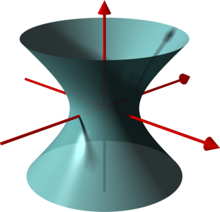
In geometry, a hyperboloid of revolution, sometimes called a circular hyperboloid, is the surface generated by rotating a hyperbola around one of its principal axes. A hyperboloid is the surface obtained from a hyperboloid of revolution by deforming it by means of directional scalings, or more generally, of an affine transformation.

<span class="mw-page-title-main">Hyperbolic geometry</span> Non-Euclidean geometry

In mathematics, hyperbolic geometry is a non-Euclidean geometry. The parallel postulate of Euclidean geometry is replaced with:

<span class="mw-page-title-main">Gudermannian function</span> Mathematical function relating circular and hyperbolic functions

In mathematics, the Gudermannian function relates a hyperbolic angle measure to a circular angle measure called the gudermannian of and denoted . The Gudermannian function reveals a close relationship between the circular functions and hyperbolic functions. It was introduced in the 1760s by Johann Heinrich Lambert, and later named for Christoph Gudermann who also described the relationship between circular and hyperbolic functions in 1830. The gudermannian is sometimes called the hyperbolic amplitude as a limiting case of the Jacobi elliptic amplitude when parameter

<span class="mw-page-title-main">Poincaré half-plane model</span> Upper-half plane model of hyperbolic non-Euclidean geometry

In non-Euclidean geometry, the Poincaré half-plane model is the upper half-plane, denoted below as H, together with a metric, the Poincaré metric, that makes it a model of two-dimensional hyperbolic geometry.

<span class="mw-page-title-main">Tractrix</span> Curve traced by a point on a rod as one end is dragged along a line

In geometry, a tractrix is the curve along which an object moves, under the influence of friction, when pulled on a horizontal plane by a line segment attached to a pulling point that moves at a right angle to the initial line between the object and the puller at an infinitesimal speed. It is therefore a curve of pursuit. It was first introduced by Claude Perrault in 1670, and later studied by Isaac Newton (1676) and Christiaan Huygens (1693).

<span class="mw-page-title-main">Tangent half-angle formula</span> Relates the tangent of half of an angle to trigonometric functions of the entire angle

In trigonometry, tangent half-angle formulas relate the tangent of half of an angle to trigonometric functions of the entire angle. The tangent of half an angle is the stereographic projection of the circle through the point at angle radians onto the line through the angles . Among these formulas are the following:

<span class="mw-page-title-main">Hyperbolic angle</span> Argument of the hyperbolic functions

In geometry, hyperbolic angle is a real number determined by the area of the corresponding hyperbolic sector of xy = 1 in Quadrant I of the Cartesian plane. The hyperbolic angle parametrises the unit hyperbola, which has hyperbolic functions as coordinates. In mathematics, hyperbolic angle is an invariant measure as it is preserved under hyperbolic rotation.

<span class="mw-page-title-main">Angle of parallelism</span> An angle in certain right triangles in the hyperbolic plane

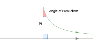
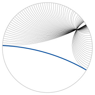
In hyperbolic geometry, angle of parallelism is the angle at the non-right angle vertex of a right hyperbolic triangle having two asymptotic parallel sides. The angle depends on the segment length a between the right angle and the vertex of the angle of parallelism.

<span class="mw-page-title-main">Hyperbolic motion (relativity)</span> Motion of an object with constant proper acceleration in special relativity.

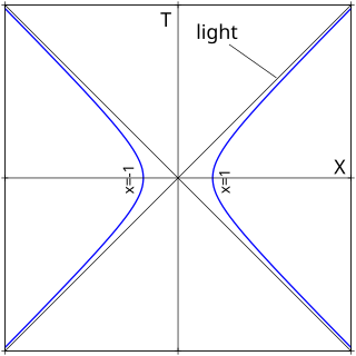
Hyperbolic motion is the motion of an object with constant proper acceleration in special relativity. It is called hyperbolic motion because the equation describing the path of the object through spacetime is a hyperbola, as can be seen when graphed on a Minkowski diagram whose coordinates represent a suitable inertial (non-accelerated) frame. This motion has several interesting features, among them that it is possible to outrun a photon if given a sufficient head start, as may be concluded from the diagram.

<span class="mw-page-title-main">Pseudorapidity</span> Spatial coordinate used in experimental particle physics

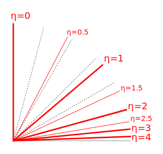
In experimental particle physics, pseudorapidity, , is a commonly used spatial coordinate describing the angle of a particle relative to the beam axis. It is defined as

<span class="mw-page-title-main">Inverse hyperbolic functions</span> Mathematical functions

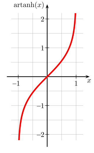
In mathematics, the inverse hyperbolic functions are inverses of the hyperbolic functions, analogous to the inverse circular functions. There are six in common use: inverse hyperbolic sine, inverse hyperbolic cosine, inverse hyperbolic tangent, inverse hyperbolic cosecant, inverse hyperbolic secant, and inverse hyperbolic cotangent. They are commonly denoted by the symbols for the hyperbolic functions, prefixed with arc- or ar-.

<span class="mw-page-title-main">Rapidity</span> Measure of relativistic velocity

Rapidity is a measure for relativistic velocity. For one-dimensional motion, rapidities are additive. However, velocities must be combined by Einstein's velocity-addition formula. For low speeds, rapidity and velocity are almost exactly proportional but, for higher velocities, rapidity takes a larger value, with the rapidity of light being infinite.

<span class="mw-page-title-main">Hyperboloid model</span> Model of n-dimensional hyperbolic geometry

In geometry, the hyperboloid model, also known as the Minkowski model after Hermann Minkowski, is a model of n-dimensional hyperbolic geometry in which points are represented by points on the forward sheet S+ of a two-sheeted hyperboloid in (n+1)-dimensional Minkowski space or by the displacement vectors from the origin to those points, and m-planes are represented by the intersections of (m+1)-planes passing through the origin in Minkowski space with S+ or by wedge products of m vectors. Hyperbolic space is embedded isometrically in Minkowski space; that is, the hyperbolic distance function is inherited from Minkowski space, analogous to the way spherical distance is inherited from Euclidean distance when the n-sphere is embedded in (n+1)-dimensional Euclidean space.

<span class="mw-page-title-main">Toroidal coordinates</span>

Toroidal coordinates are a three-dimensional orthogonal coordinate system that results from rotating the two-dimensional bipolar coordinate system about the axis that separates its two foci. Thus, the two foci and in bipolar coordinates become a ring of radius in the plane of the toroidal coordinate system; the -axis is the axis of rotation. The focal ring is also known as the reference circle.

<span class="mw-page-title-main">Oblate spheroidal coordinates</span> Three-dimensional orthogonal coordinate system

Oblate spheroidal coordinates are a three-dimensional orthogonal coordinate system that results from rotating the two-dimensional elliptic coordinate system about the non-focal axis of the ellipse, i.e., the symmetry axis that separates the foci. Thus, the two foci are transformed into a ring of radius in the x-y plane. Oblate spheroidal coordinates can also be considered as a limiting case of ellipsoidal coordinates in which the two largest semi-axes are equal in length.

<span class="mw-page-title-main">Poincaré disk model</span> Model of hyperbolic geometry

In geometry, the Poincaré disk model, also called the conformal disk model, is a model of 2-dimensional hyperbolic geometry in which all points are inside the unit disk, and straight lines are either circular arcs contained within the disk that are orthogonal to the unit circle or diameters of the unit circle.

<span class="mw-page-title-main">Integral of the secant function</span> Antiderivative of the secant function

In calculus, the integral of the secant function can be evaluated using a variety of methods and there are multiple ways of expressing the antiderivative, all of which can be shown to be equivalent via trigonometric identities,

References

  1. 1 2 3 4 5 Martin, George E. (1998). The foundations of geometry and the non-Euclidean plane (Corrected 4. print. ed.). New York, NY: Springer. pp.  447–450. ISBN   0387906940.
  2. Smorgorzhevsky, A.S. (1982). Lobachevskian geometry. Moscow: Mir. pp. 64–68.
  3. Ramsay, Arlan; Richtmyer, Robert D. (1995). Introduction to hyperbolic geometry . New York: Springer-Verlag. pp.  97–103. ISBN   0387943390.
  4. Hyperbolic Barycentric Coordinates, Abraham A. Ungar, The Australian Journal of Mathematical Analysis and Applications, AJMAA, Volume 6, Issue 1, Article 18, pp. 1–35, 2009
  5. Hyperbolic Triangle Centers: The Special Relativistic Approach, Abraham Ungar, Springer, 2010
  6. Barycentric Calculus In Euclidean And Hyperbolic Geometry: A Comparative Introduction Archived 2012-05-19 at the Wayback Machine , Abraham Ungar, World Scientific, 2010