In mathematical analysis, semicontinuity is a property of extended real-valued functions that is weaker than continuity. An extended real-valued function is uppersemicontinuous at a point if, roughly speaking, the function values for arguments near are not much higher than
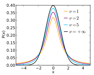
In probability and statistics, Student's t-distribution is any member of a family of continuous probability distributions that arise when estimating the mean of a normally distributed population in situations where the sample size is small and the population's standard deviation is unknown. It was developed by English statistician William Sealy Gosset under the pseudonym "Student".

In probability theory, the law of large numbers (LLN) is a theorem that describes the result of performing the same experiment a large number of times. According to the law, the average of the results obtained from a large number of trials should be close to the expected value and tends to become closer to the expected value as more trials are performed.
In mathematics, the moments of a function are certain quantitative measures related to the shape of the function's graph. If the function represents mass density, then the zeroth moment is the total mass, the first moment is the center of mass, and the second moment is the moment of inertia. If the function is a probability distribution, then the first moment is the expected value, the second central moment is the variance, the third standardized moment is the skewness, and the fourth standardized moment is the kurtosis. The mathematical concept is closely related to the concept of moment in physics.
In mathematics, the total variation identifies several slightly different concepts, related to the (local or global) structure of the codomain of a function or a measure. For a real-valued continuous function f, defined on an interval [a, b] ⊂ R, its total variation on the interval of definition is a measure of the one-dimensional arclength of the curve with parametric equation x ↦ f(x), for x ∈ [a, b]. Functions whose total variation is finite are called functions of bounded variation.
In probability and statistics, a mixture distribution is the probability distribution of a random variable that is derived from a collection of other random variables as follows: first, a random variable is selected by chance from the collection according to given probabilities of selection, and then the value of the selected random variable is realized. The underlying random variables may be random real numbers, or they may be random vectors, in which case the mixture distribution is a multivariate distribution.
In statistics, sometimes the covariance matrix of a multivariate random variable is not known but has to be estimated. Estimation of covariance matrices then deals with the question of how to approximate the actual covariance matrix on the basis of a sample from the multivariate distribution. Simple cases, where observations are complete, can be dealt with by using the sample covariance matrix. The sample covariance matrix (SCM) is an unbiased and efficient estimator of the covariance matrix if the space of covariance matrices is viewed as an extrinsic convex cone in Rp×p; however, measured using the intrinsic geometry of positive-definite matrices, the SCM is a biased and inefficient estimator. In addition, if the random variable has a normal distribution, the sample covariance matrix has a Wishart distribution and a slightly differently scaled version of it is the maximum likelihood estimate. Cases involving missing data, heteroscedasticity, or autocorrelated residuals require deeper considerations. Another issue is the robustness to outliers, to which sample covariance matrices are highly sensitive.
The algebra of random variables in statistics, provides rules for the symbolic manipulation of random variables, while avoiding delving too deeply into the mathematically sophisticated ideas of probability theory. Its symbolism allows the treatment of sums, products, ratios and general functions of random variables, as well as dealing with operations such as finding the probability distributions and the expectations, variances and covariances of such combinations.
In probability theory and statistics, the generalized extreme value (GEV) distribution is a family of continuous probability distributions developed within extreme value theory to combine the Gumbel, Fréchet and Weibull families also known as type I, II and III extreme value distributions. By the extreme value theorem the GEV distribution is the only possible limit distribution of properly normalized maxima of a sequence of independent and identically distributed random variables. Note that a limit distribution needs to exist, which requires regularity conditions on the tail of the distribution. Despite this, the GEV distribution is often used as an approximation to model the maxima of long (finite) sequences of random variables.

In probability theory and directional statistics, the von Mises distribution is a continuous probability distribution on the circle. It is a close approximation to the wrapped normal distribution, which is the circular analogue of the normal distribution. A freely diffusing angle on a circle is a wrapped normally distributed random variable with an unwrapped variance that grows linearly in time. On the other hand, the von Mises distribution is the stationary distribution of a drift and diffusion process on the circle in a harmonic potential, i.e. with a preferred orientation. The von Mises distribution is the maximum entropy distribution for circular data when the real and imaginary parts of the first circular moment are specified. The von Mises distribution is a special case of the von Mises–Fisher distribution on the N-dimensional sphere.
Imprecise probability generalizes probability theory to allow for partial probability specifications, and is applicable when information is scarce, vague, or conflicting, in which case a unique probability distribution may be hard to identify. Thereby, the theory aims to represent the available knowledge more accurately. Imprecision is useful for dealing with expert elicitation, because:
In mathematics — specifically, in large deviations theory — a rate function is a function used to quantify the probabilities of rare events. It is required to have several properties which assist in the formulation of the large deviation principle. In some sense, the large deviation principle is an analogue of weak convergence of probability measures, but one which takes account of how well the rare events behave.
In mathematics, more specifically measure theory, there are various notions of the convergence of measures. For an intuitive general sense of what is meant by convergence of measures, consider a sequence of measures μn on a space, sharing a common collection of measurable sets. Such a sequence might represent an attempt to construct 'better and better' approximations to a desired measure μ that is difficult to obtain directly. The meaning of 'better and better' is subject to all the usual caveats for taking limits; for any error tolerance ε > 0 we require there be N sufficiently large for n ≥ N to ensure the 'difference' between μn and μ is smaller than ε. Various notions of convergence specify precisely what the word 'difference' should mean in that description; these notions are not equivalent to one another, and vary in strength.

In numerical analysis, the interval finite element method is a finite element method that uses interval parameters. Interval FEM can be applied in situations where it is not possible to get reliable probabilistic characteristics of the structure. This is important in concrete structures, wood structures, geomechanics, composite structures, biomechanics and in many other areas. The goal of the Interval Finite Element is to find upper and lower bounds of different characteristics of the model and use these results in the design process. This is so called worst case design, which is closely related to the limit state design.
In mathematics, the Pettis integral or Gelfand–Pettis integral, named after Israel M. Gelfand and Billy James Pettis, extends the definition of the Lebesgue integral to vector-valued functions on a measure space, by exploiting duality. The integral was introduced by Gelfand for the case when the measure space is an interval with Lebesgue measure. The integral is also called the weak integral in contrast to the Bochner integral, which is the strong integral.
In probability theory, the family of complex normal distributions, denoted or , characterizes complex random variables whose real and imaginary parts are jointly normal. The complex normal family has three parameters: location parameter μ, covariance matrix , and the relation matrix . The standard complex normal is the univariate distribution with , , and .

In mathematics, the integral of a non-negative function of a single variable can be regarded, in the simplest case, as the area between the graph of that function and the x-axis. The Lebesgue integral, named after French mathematician Henri Lebesgue, extends the integral to a larger class of functions. It also extends the domains on which these functions can be defined.

A probability box is a characterization of uncertain numbers consisting of both aleatoric and epistemic uncertainties that is often used in risk analysis or quantitative uncertainty modeling where numerical calculations must be performed. Probability bounds analysis is used to make arithmetic and logical calculations with p-boxes.
Credal networks are probabilistic graphical models based on imprecise probability. Credal networks can be regarded as an extension of Bayesian networks, where credal sets replace probability mass functions in the specification of the local models for the network variables given their parents. As a Bayesian network defines a joint probability mass function over its variables, a credal network defines a joint credal set. The way this credal set is defined depends on the particular notion of independence for imprecise probability adopted. Most of the research on credal networks focused on the case of strong independence. Given strong independence the joint credal set associated to a credal network is called its strong extension. Let denote a collection of categorical variables and . If is, for each , a conditional credal set over , then the strong extension of a credal network is defined as follows:
In probability theory and statistics, the Dirichlet process (DP) is one of the most popular Bayesian nonparametric models. It was introduced by Thomas Ferguson as a prior over probability distributions.


