Cubic Hermite spline

Last updated

In numerical analysis, a cubic Hermite spline or cubic Hermite interpolator is a spline where each piece is a third-degree polynomial specified in Hermite form, that is, by its values and first derivatives at the end points of the corresponding domain interval. [1]

Contents

Cubic Hermite splines are typically used for interpolation of numeric data specified at given argument values , to obtain a continuous function. The data should consist of the desired function value and derivative at each . (If only the values are provided, the derivatives must be estimated from them.) The Hermite formula is applied to each interval separately. The resulting spline will be continuous and will have continuous first derivative.

Cubic polynomial splines can be specified in other ways, the Bezier cubic being the most common. However, these two methods provide the same set of splines, and data can be easily converted between the Bézier and Hermite forms; so the names are often used as if they were synonymous.

Cubic polynomial splines are extensively used in computer graphics and geometric modeling to obtain curves or motion trajectories that pass through specified points of the plane or three-dimensional space. In these applications, each coordinate of the plane or space is separately interpolated by a cubic spline function of a separate parameter t. Cubic polynomial splines are also used extensively in structural analysis applications, such as Euler–Bernoulli beam theory. Cubic polynomial splines have also been applied to mortality analysis [2] and mortality forecasting. [3]

Cubic splines can be extended to functions of two or more parameters, in several ways. Bicubic splines (Bicubic interpolation) are often used to interpolate data on a regular rectangular grid, such as pixel values in a digital image or altitude data on a terrain. Bicubic surface patches, defined by three bicubic splines, are an essential tool in computer graphics.

Cubic splines are often called csplines, especially in computer graphics. Hermite splines are named after Charles Hermite.

Interpolation on a single interval

Unit interval [0, 1]

The four Hermite basis functions. The interpolant in each subinterval is a linear combination of these four functions. HermiteBasis.svg
The four Hermite basis functions. The interpolant in each subinterval is a linear combination of these four functions.

On the unit interval , given a starting point at and an ending point at with starting tangent at and ending tangent at , the polynomial can be defined by

where t ∈ [0, 1].

Interpolation on an arbitrary interval

Interpolating in an arbitrary interval is done by mapping the latter to through an affine (degree-1) change of variable. The formula is

where , and refers to the basis functions, defined below. Note that the tangent values have been scaled by compared to the equation on the unit interval.

Uniqueness

The formula specified above provides the unique third-degree polynomial path between the two points with the given tangents.

Proof. Let be two third-degree polynomials satisfying the given boundary conditions. Define then:

Since both and are third-degree polynomials, is at most a third-degree polynomial. So must be of the form

Calculating the derivative gives

We know furthermore that


(1)


(2)

Putting ( 1 ) and ( 2 ) together, we deduce that , and therefore thus

Representations

We can write the interpolation polynomial as

where , , , are Hermite basis functions. These can be written in different ways, each way revealing different properties:

expanded factorized Bernstein

The "expanded" column shows the representation used in the definition above. The "factorized" column shows immediately that and are zero at the boundaries. You can further conclude that and have a zero of multiplicity 2 at 0, and and have such a zero at 1, thus they have slope 0 at those boundaries. The "Bernstein" column shows the decomposition of the Hermite basis functions into Bernstein polynomials of order 3:

Using this connection you can express cubic Hermite interpolation in terms of cubic Bézier curves with respect to the four values and do Hermite interpolation using the de Casteljau algorithm. It shows that in a cubic Bézier patch the two control points in the middle determine the tangents of the interpolation curve at the respective outer points.

We can also write the polynomial in standard form as

where the control points and tangents are coefficients. This permits efficient evaluation of the polynomial at various values of t since the constant coefficients can be computed once and reused.

Interpolating a data set

A data set, for , can be interpolated by applying the above procedure on each interval, where the tangents are chosen in a sensible manner, meaning that the tangents for intervals sharing endpoints are equal. The interpolated curve then consists of piecewise cubic Hermite splines and is globally continuously differentiable in .

The choice of tangents is not unique, and there are several options available.

Finite difference

Example with finite-difference tangents Finite difference spline example.png
Example with finite-difference tangents

The simplest choice is the three-point difference, not requiring constant interval lengths:

for internal points , and one-sided difference at the endpoints of the data set.

Cardinal spline

Cardinal spline example in 2D. The line represents the curve, and the squares represent the control points
p
k
{\displaystyle {\boldsymbol {p}}_{k}}
. Notice that the curve does not reach the first and last points; these points do, however, affect the shape of the curve. The tension parameter used is 0.1 Cardinal Spline Example.png
Cardinal spline example in 2D. The line represents the curve, and the squares represent the control points . Notice that the curve does not reach the first and last points; these points do, however, affect the shape of the curve. The tension parameter used is 0.1

A cardinal spline, sometimes called a canonical spline, [4] is obtained [5] if

is used to calculate the tangents. The parameter c is a tension parameter that must be in the interval [0, 1]. In some sense, this can be interpreted as the "length" of the tangent. Choosing c = 1 yields all zero tangents, and choosing c = 0 yields a Catmull–Rom spline in the uniform parameterization case.

Catmull–Rom spline

Geometric interpretation of Catmull-Rom cubic interpolation of the black point with uniformly spaced abscissae. Cubic interpolation visualisation.svg
Geometric interpretation of Catmull–Rom cubic interpolation of the black point with uniformly spaced abscissae.

For tangents chosen to be

a Catmull–Rom spline is obtained, being a special case of a cardinal spline. This assumes uniform parameter spacing.

The curve is named after Edwin Catmull and Raphael Rom. The principal advantage of this technique is that the points along the original set of points also make up the control points for the spline curve. [7] Two additional points are required on either end of the curve. The uniform Catmull–Rom implementation can produce loops and self-intersections. The chordal and centripetal Catmull–Rom implementations [8] solve this problem, but use a slightly different calculation. [9] In computer graphics, Catmull–Rom splines are frequently used to get smooth interpolated motion between key frames. For example, most camera path animations generated from discrete key-frames are handled using Catmull–Rom splines. They are popular mainly for being relatively easy to compute, guaranteeing that each key frame position will be hit exactly, and also guaranteeing that the tangents of the generated curve are continuous over multiple segments.

Kochanek–Bartels spline

A Kochanek–Bartels spline is a further generalization on how to choose the tangents given the data points , and , with three parameters possible: tension, bias and a continuity parameter.

Monotone cubic interpolation

If a cubic Hermite spline of any of the above listed types is used for interpolation of a monotonic data set, the interpolated function will not necessarily be monotonic, but monotonicity can be preserved by adjusting the tangents.

Interpolation on the unit interval with matched derivatives at endpoints

Consider a single coordinate of the points and as the values that a function f(x) takes at integer ordinates x = n  1, n, n + 1 and n + 2,

In addition, assume that the tangents at the endpoints are defined as the centered differences of the adjacent points:

To evaluate the interpolated f(x) for a real x, first separate x into the integer portion n and fractional portion u:

where denotes the floor function, which returns the largest integer no larger than x.

Then the Catmull–Rom spline is [10]

where denotes the matrix transpose. The bottom equality is depicting the application of Horner's method.

This writing is relevant for tricubic interpolation, where one optimization requires computing CINTu sixteen times with the same u and different p.

See also

Related Research Articles

<span class="mw-page-title-main">Interpolation</span> Method for estimating new data within known data points

In the mathematical field of numerical analysis, interpolation is a type of estimation, a method of constructing (finding) new data points based on the range of a discrete set of known data points.

<span class="mw-page-title-main">B-spline</span> Spline function

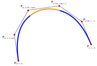
In the mathematical subfield of numerical analysis, a B-spline or basis spline is a spline function that has minimal support with respect to a given degree, smoothness, and domain partition. Any spline function of given degree can be expressed as a linear combination of B-splines of that degree. Cardinal B-splines have knots that are equidistant from each other. B-splines can be used for curve-fitting and numerical differentiation of experimental data.

<span class="mw-page-title-main">Ellipsoid</span> Quadric surface that looks like a deformed sphere

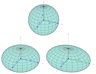
An ellipsoid is a surface that can be obtained from a sphere by deforming it by means of directional scalings, or more generally, of an affine transformation.

In mathematics, the Hermite polynomials are a classical orthogonal polynomial sequence.

In numerical analysis, polynomial interpolation is the interpolation of a given bivariate data set by the polynomial of lowest possible degree that passes through the points of the dataset.

In the mathematical field of numerical analysis, a Newton polynomial, named after its inventor Isaac Newton, is an interpolation polynomial for a given set of data points. The Newton polynomial is sometimes called Newton's divided differences interpolation polynomial because the coefficients of the polynomial are calculated using Newton's divided differences method.

<span class="mw-page-title-main">Lagrange polynomial</span> Polynomials used for interpolation

In numerical analysis, the Lagrange interpolating polynomial is the unique polynomial of lowest degree that interpolates a given set of data.

<span class="mw-page-title-main">Spline (mathematics)</span> Mathematical function defined piecewise by polynomials

In mathematics, a spline is a function defined piecewise by polynomials. In interpolating problems, spline interpolation is often preferred to polynomial interpolation because it yields similar results, even when using low degree polynomials, while avoiding Runge's phenomenon for higher degrees.

In the mathematical field of numerical analysis, spline interpolation is a form of interpolation where the interpolant is a special type of piecewise polynomial called a spline. That is, instead of fitting a single, high-degree polynomial to all of the values at once, spline interpolation fits low-degree polynomials to small subsets of the values, for example, fitting nine cubic polynomials between each of the pairs of ten points, instead of fitting a single degree-nine polynomial to all of them. Spline interpolation is often preferred over polynomial interpolation because the interpolation error can be made small even when using low-degree polynomials for the spline. Spline interpolation also avoids the problem of Runge's phenomenon, in which oscillation can occur between points when interpolating using high-degree polynomials.

<span class="mw-page-title-main">Sinc function</span> Special mathematical function defined as sin(x)/x

In mathematics, physics and engineering, the sinc function, denoted by sinc(x), has two forms, normalized and unnormalized.

<span class="mw-page-title-main">Kochanek–Bartels spline</span>

In mathematics, a Kochanek–Bartels spline or Kochanek–Bartels curve is a cubic Hermite spline with tension, bias, and continuity parameters defined to change the behavior of the tangents.

In mathematics, trigonometric interpolation is interpolation with trigonometric polynomials. Interpolation is the process of finding a function which goes through some given data points. For trigonometric interpolation, this function has to be a trigonometric polynomial, that is, a sum of sines and cosines of given periods. This form is especially suited for interpolation of periodic functions.

<span class="mw-page-title-main">Bicubic interpolation</span> Extension of cubic spline interpolation

In mathematics, bicubic interpolation is an extension of cubic spline interpolation for interpolating data points on a two-dimensional regular grid. The interpolated surface is smoother than corresponding surfaces obtained by bilinear interpolation or nearest-neighbor interpolation. Bicubic interpolation can be accomplished using either Lagrange polynomials, cubic splines, or cubic convolution algorithm.

In mathematics, Birkhoff interpolation is an extension of polynomial interpolation. It refers to the problem of finding a polynomial of degree such that only certain derivatives have specified values at specified points:

In numerical analysis, Hermite interpolation, named after Charles Hermite, is a method of polynomial interpolation, which generalizes Lagrange interpolation. Lagrange interpolation allows computing a polynomial of degree less than n that takes the same value at n given points as a given function. Instead, Hermite interpolation computes a polynomial of degree less than mn such that the polynomial and its first m − 1 derivatives have the same values at n given points as a given function and its first m − 1 derivatives.

In applied mathematics, polyharmonic splines are used for function approximation and data interpolation. They are very useful for interpolating and fitting scattered data in many dimensions. Special cases include thin plate splines and natural cubic splines in one dimension.

In the mathematical field of numerical analysis, monotone cubic interpolation is a variant of cubic interpolation that preserves monotonicity of the data set being interpolated.

In numerical analysis, multivariate interpolation is interpolation on functions of more than one variable ; when the variates are spatial coordinates, it is also known as spatial interpolation.

In mathematics, a set of n functions f1, f2, ..., fn is unisolvent on a domain Ω if the vectors

Image derivatives can be computed by using small convolution filters of size 2 × 2 or 3 × 3, such as the Laplacian, Sobel, Roberts and Prewitt operators. However, a larger mask will generally give a better approximation of the derivative and examples of such filters are Gaussian derivatives and Gabor filters. Sometimes high frequency noise needs to be removed and this can be incorporated in the filter so that the Gaussian kernel will act as a band pass filter. The use of Gabor filters in image processing has been motivated by some of its similarities to the perception in the human visual system.

References

  1. Erwin Kreyszig (2005). Advanced Engineering Mathematics (9 ed.). Wiley. p. 816. ISBN   9780471488859.
  2. Stephen Richards (2020). "A Hermite-spline model of post-retirement mortality". Scandinavian Actuarial Journal. Taylor and Francis: 110–127. doi:10.1080/03461238.2019.1642239.
  3. Sixian Tang, Jackie Li and Leonie Tickle (2022). "A Hermite spline approach for modelling population mortality". Annals of Actuarial Science. Cambridge University Press: 1–42. doi:10.1017/S1748499522000173.
  4. Petzold, Charles (2009). "Canonical Splines in WPF and Silverlight".
  5. "Cardinal Splines". Microsoft Developer Network. Retrieved 2018-05-27.
  6. Cubic interpolation is not unique: this model using a Catmull-Rom spline and Lagrange basis polynomials passes through all four points. Note: If the black point is left of the yellow point, the yellow horizontal distance is negative; if the black point is on the right of the green point, the green horizontal distance is negative.
  7. Catmull, Edwin; Rom, Raphael (1974), "A class of local interpolating splines", in Barnhill, R. E.; Riesenfeld, R. F. (eds.), Computer Aided Geometric Design, New York: Academic Press, pp. 317–326
  8. N. Dyn, M. S. Floater, and K. Hormann. Four-point curve subdivision based on iterated chordal and centripetal parameterizations. Computer Aided Geometric Design, 26(3):279–286, 2009.
  9. P. J. Barry and R. N. Goldman. A recursive evaluation algorithm for a class of Catmull-Rom splines. SIGGRAPH Computer Graphics, 22(4):199–204, 1988.
  10. Two hierarchies of spline interpolations. Practical algorithms for multivariate higher order splines.