Data-driven control system

Last updated April 28, 2024

Data-driven control systems are a broad family of control systems, in which the identification of the process model and/or the design of the controller are based entirely on experimental data collected from the plant.^[1]

In many control applications, trying to write a mathematical model of the plant is considered a hard task, requiring efforts and time to the process and control engineers. This problem is overcome by data-driven methods, which fit a system model to the experimental data collected, choosing it in a specific models class. The control engineer can then exploit this model to design a proper controller for the system. However, it is still difficult to find a simple yet reliable model for a physical system, that includes only those dynamics of the system that are of interest for the control specifications. The direct data-driven methods allow to tune a controller, belonging to a given class, without the need of an identified model of the system. In this way, one can also simply weight process dynamics of interest inside the control cost function, and exclude those dynamics that are out of interest.

Overview

The standard approach to control systems design is organized in two-steps:

Model identification aims at estimating a nominal model of the system ${\widehat {G}}=G\left(q;{\widehat {\theta }}_{N}\right)$ , where $q$ is the unit-delay operator (for discrete-time transfer functions representation) and ${\widehat {\theta }}_{N}$ is the vector of parameters of $G$ identified on a set of $N$ data. Then, validation consists in constructing the uncertainty set $\Gamma$ that contains the true system $G_{0}$ at a certain probability level.
Controller design aims at finding a controller $C$ achieving closed-loop stability and meeting the required performance with ${\widehat {G}}$ .

Typical objectives of system identification are to have ${\widehat {G}}$ as close as possible to $G_{0}$ , and to have $\Gamma$ as small as possible. However, from an identification for control perspective, what really matters is the performance achieved by the controller, not the intrinsic quality of the model.

One way to deal with uncertainty is to design a controller that has an acceptable performance with all models in $\Gamma$ , including $G_{0}$ . This is the main idea behind robust control design procedure, that aims at building frequency domain uncertainty descriptions of the process. However, being based on worst-case assumptions rather than on the idea of averaging out the noise, this approach typically leads to conservative uncertainty sets. Rather, data-driven techniques deal with uncertainty by working on experimental data, and avoiding excessive conservativism.

In the following, the main classifications of data-driven control systems are presented.

Indirect and direct methods

There are many methods available to control the systems. The fundamental distinction is between indirect and direct controller design methods. The former group of techniques is still retaining the standard two-step approach, i.e. first a model is identified, then a controller is tuned based on such model. The main issue in doing so is that the controller is computed from the estimated model ${\widehat {G}}$ (according to the certainty equivalence principle), but in practice ${\widehat {G}}\neq G_{0}$ . To overcome this problem, the idea behind the latter group of techniques is to map the experimental data directly onto the controller, without any model to be identified in between.

Iterative and noniterative methods

Another important distinction is between iterative and noniterative (or one-shot) methods. In the former group, repeated iterations are needed to estimate the controller parameters, during which the optimization problem is performed based on the results of the previous iteration, and the estimation is expected to become more and more accurate at each iteration. This approach is also prone to on-line implementations (see below). In the latter group, the (optimal) controller parametrization is provided with a single optimization problem. This is particularly important for those systems in which iterations or repetitions of data collection experiments are limited or even not allowed (for example, due to economic aspects). In such cases, one should select a design technique capable of delivering a controller on a single data set. This approach is often implemented off-line (see below).

On-line and off-line methods

Since, on practical industrial applications, open-loop or closed-loop data are often available continuously, on-line data-driven techniques use those data to improve the quality of the identified model and/or the performance of the controller each time new information is collected on the plant. Instead, off-line approaches work on batch of data, which may be collected only once, or multiple times at a regular (but rather long) interval of time.

Iterative feedback tuning

The iterative feedback tuning (IFT) method was introduced in 1994,^[2] starting from the observation that, in identification for control, each iteration is based on the (wrong) certainty equivalence principle.

IFT is a model-free technique for the direct iterative optimization of the parameters of a fixed-order controller; such parameters can be successively updated using information coming from standard (closed-loop) system operation.

Let $y^{d}$ be a desired output to the reference signal $r$ ; the error between the achieved and desired response is ${\tilde {y}}(\rho )=y(\rho )-y^{d}$ . The control design objective can be formulated as the minimization of the objective function:

J(\rho )={\frac {1}{2N}}\sum _{t=1}^{N}E\left[{\tilde {y}}(t,\rho )^{2}\right].

Given the objective function to minimize, the quasi-Newton method can be applied, i.e. a gradient-based minimization using a gradient search of the type:

\rho _{i+1}=\rho _{i}-\gamma _{i}R_{i}^{-1}{\frac {d{\widehat {J}}}{d\rho }}(\rho _{i}).

The value $\gamma _{i}$ is the step size, $R_{i}$ is an appropriate positive definite matrix and ${\frac {d{\widehat {J}}}{d\rho }}$ is an approximation of the gradient; the true value of the gradient is given by the following:

{\frac {dJ}{d\rho }}(\rho )={\frac {1}{N}}\sum _{t=1}^{N}\left[{\tilde {y}}(t,\rho ){\frac {\delta y}{\delta \rho }}(t,\rho )\right].

The value of ${\frac {\delta y}{\delta \rho }}(t,\rho )$ is obtained through the following three-step methodology:

Normal Experiment: Perform an experiment on the closed loop system with $C(\rho )$ as controller and $r$ as reference; collect N measurements of the output $y(\rho )$ , denoted as $y^{(1)}(\rho )$ .
Gradient Experiment: Perform an experiment on the closed loop system with $C(\rho )$ as controller and 0 as reference $r$ ; inject the signal $r-y^{(1)}(\rho )$ such that it is summed to the control variable output by $C(\rho )$ , going as input into the plant. Collect the output, denoted as $y^{(2)}(\rho )$ .
Take the following as gradient approximation: ${\frac {\delta {\widehat {y}}}{\delta \rho }}(\rho )={\frac {\delta C}{\delta \rho }}(\rho )y^{(2)}(\rho )$ .

A crucial factor for the convergence speed of the algorithm is the choice of $R_{i}$ ; when ${\tilde {y}}$ is small, a good choice is the approximation given by the Gauss–Newton direction:

R_{i}={\frac {1}{N}}\sum _{t=1}^{N}{\frac {\delta {\widehat {y}}}{\delta \rho }}(\rho _{i}){\frac {\delta {\widehat {y}}^{T}}{\delta \rho }}(\rho _{i}).

Noniterative correlation-based tuning

Noniterative correlation-based tuning (nCbT) is a noniterative method for data-driven tuning of a fixed-structure controller.^[3] It provides a one-shot method to directly synthesize a controller based on a single dataset.

Suppose that $G$ denotes an unknown LTI stable SISO plant, $M$ a user-defined reference model and $F$ a user-defined weighting function. An LTI fixed-order controller is indicated as $K(\rho )=\beta ^{T}\rho$ , where $\rho \in \mathbb {R} ^{n}$ , and $\beta$ is a vector of LTI basis functions. Finally, $K^{*}$ is an ideal LTI controller of any structure, guaranteeing a closed-loop function $M$ when applied to $G$ .

The goal is to minimize the following objective function:

J(\rho )=\left\|F{\bigg (}{\frac {K^{*}G-K(\rho )G}{(1+K^{*}G)^{2}}}{\bigg )}\right\|_{2}^{2}.

$J(\rho )$ is a convex approximation of the objective function obtained from a model reference problem, supposing that ${\frac {1}{(1+K(\rho )G)}}\approx {\frac {1}{(1+K^{*}G)}}$ .

When $G$ is stable and minimum-phase, the approximated model reference problem is equivalent to the minimization of the norm of $\varepsilon (t)$ in the scheme in figure.

The input signal $r(t)$ is supposed to be a persistently exciting input signal and $v(t)$ to be generated by a stable data-generation mechanism. The two signals are thus uncorrelated in an open-loop experiment; hence, the ideal error $\varepsilon (t,\rho ^{*})$ is uncorrelated with $r(t)$ . The control objective thus consists in finding $\rho$ such that $r(t)$ and $\varepsilon (t,\rho ^{*})$ are uncorrelated.

The vector of instrumental variables $\zeta (t)$ is defined as:

\zeta (t)=[r_{W}(t+\ell _{1}),r_{W}(t+\ell _{1}-1),\ldots ,r_{W}(t),\ldots ,r_{W}(t-\ell _{1})]^{T}

where $\ell _{1}$ is large enough and $r_{W}(t)=Wr(t)$ , where $W$ is an appropriate filter.

The correlation function is:

f_{N,\ell _{1}}(\rho )={\frac {1}{N}}\sum _{t=1}^{N}\zeta (t)\varepsilon (t,\rho )

and the optimization problem becomes:

{\widehat {\rho }}={\underset {\rho \in D_{k}}{\operatorname {arg\,min} }}J_{N,\ell _{1}}(\rho )={\underset {\rho \in D_{k}}{\operatorname {arg\,min} }}f_{N,\ell _{1}}^{T}f_{N,\ell _{1}}.

Denoting with $\phi _{r}(\omega )$ the spectrum of $r(t)$ , it can be demonstrated that, under some assumptions, if $W$ is selected as:

W(e^{-j\omega })={\frac {F(e^{-j\omega })(1-M(e^{-j\omega }))}{\phi _{r}(\omega )}}

then, the following holds:

\lim _{N,\ell _{1}\to \infty ,\ell _{1}/N\to \infty }{\widehat {\rho }}=\rho ^{*}.

Stability constraint

There is no guarantee that the controller $K$ that minimizes $J_{N,\ell _{1}}$ is stable. Instability may occur in the following cases:

If $G$ is non-minimum phase, $K^{*}$ may lead to cancellations in the right-half complex plane.
If $K^{*}$ (even if stabilizing) is not achievable, $K(\rho )$ may not be stabilizing.
Due to measurement noise, even if $K^{*}=K(\rho )$ is stabilizing, data-estimated ${\widehat {K}}(\rho )$ may not be so.

Consider a stabilizing controller $K_{s}$ and the closed loop transfer function $M_{s}={\frac {K_{s}G}{1+K_{s}G}}$ . Define:

\Delta (\rho ):=M_{s}-K(\rho )G(1-M_{s})

\delta (\rho ):=\left\|\Delta (\rho )\right\|_{\infty }.

Theorem

The controller $K(\rho )$ stabilizes the plant $G$ if

$\Delta (\rho )$ is stable
$\exists \delta _{N}\in (0,1)$ s.t. $\delta (\rho )\leq \delta _{N}.$

Condition 1. is enforced when:

$K(\rho )$ is stable
$K(\rho )$ contains an integrator (it is canceled).

The model reference design with stability constraint becomes:

\rho _{s}={\underset {\rho \in D_{k}}{\operatorname {arg\,min} }}J(\rho )

{\text{s.t. }}\delta (\rho )\leq \delta _{N}.

A convex data-driven estimation of $\delta (\rho )$ can be obtained through the discrete Fourier transform.

Define the following:

{\begin{aligned}&{\widehat {R}}_{r}(\tau )={\frac {1}{N}}\sum _{t=1}^{N}r(t-\tau )r(t){\text{ for }}\tau =-\ell _{2},\ldots ,\ell _{2}\\[4pt]&{\widehat {R}}_{r\varepsilon }(\tau )={\frac {1}{N}}\sum _{t=1}^{N}r(t-\tau )\varepsilon (t,\rho ){\text{ for }}\tau =-\ell _{2},\ldots ,\ell _{2}.\end{aligned}}

For stable minimum phase plants, the following convex data-driven optimization problem is given:

{\begin{aligned}{\widehat {\rho }}&={\underset {\rho \in D_{k}}{\operatorname {arg\,min} }}J_{N,\ell _{1}}(\rho )\\[3pt]&{\text{s.t.}}\\[3pt]&{\bigg |}\sum _{\tau =-\ell _{2}}^{\ell _{2}}{\widehat {R}}_{r\varepsilon }(\tau ,\rho )e^{-j\tau \omega _{k}}{\bigg |}\leq \delta _{N}{\bigg |}\sum _{\tau =-\ell _{2}}^{\ell _{2}}{\widehat {R}}_{r}(\tau ,\rho )e^{-j\tau \omega _{k}}{\bigg |}\\[4pt]\omega _{k}&={\frac {2\pi k}{2\ell _{2}+1}},\qquad k=0,\ldots ,\ell _{2}+1.\end{aligned}}

Virtual reference feedback tuning

Virtual Reference Feedback Tuning (VRFT) is a noniterative method for data-driven tuning of a fixed-structure controller. It provides a one-shot method to directly synthesize a controller based on a single dataset.

VRFT was first proposed in ^[4] and then extended to LPV systems.^[5] VRFT also builds on ideas given in ^[6] as $VRD^{2}$ .

The main idea is to define a desired closed loop model $M$ and to use its inverse dynamics to obtain a virtual reference $r_{v}(t)$ from the measured output signal $y(t)$ .

The virtual signals are $r_{v}(t)=M^{-1}y(t)$ and $e_{v}(t)=r_{v}(t)-y(t).$

The optimal controller is obtained from noiseless data by solving the following optimization problem:

{\widehat {\rho }}_{\infty }={\underset {\rho }{\operatorname {arg\,min} }}\lim _{N\to \infty }J_{vr}(\rho )

where the optimization function is given as follows:

J_{vr}^{N}(\rho )={\frac {1}{N}}\sum _{t=1}^{N}\left(u(t)-K(\rho )e_{v}(t)\right)^{2}.

Related Research Articles

In fluid mechanics, the Grashof number is a dimensionless number which approximates the ratio of the buoyancy to viscous forces acting on a fluid. It frequently arises in the study of situations involving natural convection and is analogous to the Reynolds number.

<span class="mw-page-title-main">Boundary layer</span> Layer of fluid in the immediate vicinity of a bounding surface

In physics and fluid mechanics, a boundary layer is the thin layer of fluid in the immediate vicinity of a bounding surface formed by the fluid flowing along the surface. The fluid's interaction with the wall induces a no-slip boundary condition. The flow velocity then monotonically increases above the surface until it returns to the bulk flow velocity. The thin layer consisting of fluid whose velocity has not yet returned to the bulk flow velocity is called the velocity boundary layer.

Linear elasticity is a mathematical model of how solid objects deform and become internally stressed due to prescribed loading conditions. It is a simplification of the more general nonlinear theory of elasticity and a branch of continuum mechanics.

The representation theory of groups is a part of mathematics which examines how groups act on given structures.

In physics, the Hamilton–Jacobi equation, named after William Rowan Hamilton and Carl Gustav Jacob Jacobi, is an alternative formulation of classical mechanics, equivalent to other formulations such as Newton's laws of motion, Lagrangian mechanics and Hamiltonian mechanics.

Large eddy simulation (LES) is a mathematical model for turbulence used in computational fluid dynamics. It was initially proposed in 1963 by Joseph Smagorinsky to simulate atmospheric air currents, and first explored by Deardorff (1970). LES is currently applied in a wide variety of engineering applications, including combustion, acoustics, and simulations of the atmospheric boundary layer.

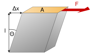
In materials science, shear modulus or modulus of rigidity, denoted by G, or sometimes S or μ, is a measure of the elastic shear stiffness of a material and is defined as the ratio of shear stress to the shear strain:

The Wigner distribution function (WDF) is used in signal processing as a transform in time-frequency analysis.

The Newman–Penrose (NP) formalism is a set of notation developed by Ezra T. Newman and Roger Penrose for general relativity (GR). Their notation is an effort to treat general relativity in terms of spinor notation, which introduces complex forms of the usual variables used in GR. The NP formalism is itself a special case of the tetrad formalism, where the tensors of the theory are projected onto a complete vector basis at each point in spacetime. Usually this vector basis is chosen to reflect some symmetry of the spacetime, leading to simplified expressions for physical observables. In the case of the NP formalism, the vector basis chosen is a null tetrad: a set of four null vectors—two real, and a complex-conjugate pair. The two real members often asymptotically point radially inward and radially outward, and the formalism is well adapted to treatment of the propagation of radiation in curved spacetime. The Weyl scalars, derived from the Weyl tensor, are often used. In particular, it can be shown that one of these scalars— $in the appropriate frame—encodes the outgoing gravitational radiation of an asymptotically flat system.$

The Cebeci–Smith model, developed by Tuncer Cebeci and Apollo M. O. Smith in 1967, is a 0-equation eddy viscosity model used in computational fluid dynamics analysis of turbulence in boundary layer flows. The model gives eddy viscosity, $, as a function of the local boundary layer velocity profile. The model is suitable for high-speed flows with thin attached boundary layers, typically present in aerospace applications. Like the Baldwin-Lomax model, it is not suitable for large regions of flow separation and significant curvature or rotation. Unlike the Baldwin-Lomax model, this model requires the determination of a boundary layer edge.$

Critical state soil mechanics is the area of soil mechanics that encompasses the conceptual models representing the mechanical behavior of saturated remoulded soils based on the critical state concept. At the critical state, the relationship between forces applied in the soil (stress), and the resulting deformation resulting from this stress (strain) becomes constant. The soil will continue to deform, but the stress will no longer increase.

The Cauchy momentum equation is a vector partial differential equation put forth by Cauchy that describes the non-relativistic momentum transport in any continuum.

Laser linewidth is the spectral linewidth of a laser beam.

In the Newman–Penrose (NP) formalism of general relativity, independent components of the Ricci tensors of a four-dimensional spacetime are encoded into seven Ricci scalars which consist of three real scalars $, three complex scalars and the NP curvature scalar . Physically, Ricci-NP scalars are related with the energy-momentum distribution of the spacetime due to Einstein's field equation.$

In structural dynamics, a moving load changes the point at which the load is applied over time. Examples include a vehicle that travels across a bridge and a train moving along a track.

Menter's Shear Stress Transport turbulence model, or SST, is a widely used and robust two-equation eddy-viscosity turbulence model used in Computational Fluid Dynamics. The model combines the k-omega turbulence model and K-epsilon turbulence model such that the k-omega is used in the inner region of the boundary layer and switches to the k-epsilon in the free shear flow.

In orbital mechanics, Gauss's method is used for preliminary orbit determination from at least three observations of the orbiting body of interest at three different times. The required information are the times of observations, the position vectors of the observation points, the direction cosine vector of the orbiting body from the observation points and general physical data.

Tau functions are an important ingredient in the modern mathematical theory of integrable systems, and have numerous applications in a variety of other domains. They were originally introduced by Ryogo Hirota in his direct method approach to soliton equations, based on expressing them in an equivalent bilinear form.

In statistics, the Innovation Method provides an estimator for the parameters of stochastic differential equations given a time series of observations of the state variables. In the framework of continuous-discrete state space models, the innovation estimator is obtained by maximizing the log-likelihood of the corresponding discrete-time innovation process with respect to the parameters. The innovation estimator can be classified as a M-estimator, a quasi-maximum likelihood estimator or a prediction error estimator depending on the inferential considerations that want to be emphasized. The innovation method is a system identification technique for developing mathematical models of dynamical systems from measured data and for the optimal design of experiments.

The recharge oscillator model for El Niño–Southern Oscillation (ENSO) is a theory described for the first time in 1997 by Jin., which explains the periodical variation of the sea surface temperature (SST) and thermocline depth that occurs in the central equatorial Pacific Ocean. The physical mechanisms at the basis of this oscillation are periodical recharges and discharges of the zonal mean equatorial heat content, due to ocean-atmosphere interaction. Other theories have been proposed to model ENSO, such as the delayed oscillator, the western Pacific oscillator and the advective reflective oscillator. A unified and consistent model has been proposed by Wang in 2001, in which the recharge oscillator model is included as a particular case.

References

↑ Bazanella, A.S., Campestrini, L., Eckhard, D. (2012). Data-driven controller design: the $H_{2}$ approach. Springer, ISBN 978-94-007-2300-9, 208 pages.
↑ Hjalmarsson, H., Gevers, M., Gunnarsson, S., & Lequin, O. (1998). Iterative feedback tuning: theory and applications. IEEE control systems, 18(4), 26–41.
↑ van Heusden, K., Karimi, A. and Bonvin, D. (2011), Data-driven model reference control with asymptotically guaranteed stability. Int. J. Adapt. Control Signal Process., 25: 331–351. doi : 10.1002/acs.1212
↑ Campi, Marco C., Andrea Lecchini, and Sergio M. Savaresi. "Virtual reference feedback tuning: a direct method for the design of feedback controllers." Automatica 38.8 (2002): 1337–1346.
↑ Formentin, S., Piga, D., Tóth, R., & Savaresi, S. M. (2016). Direct learning of LPV controllers from data. Automatica, 65, 98–110.
↑ Guardabassi, Guido O., and Sergio M. Savaresi. "Approximate feedback linearization of discrete-time non-linear systems using virtual input direct design." Systems & Control Letters 32.2 (1997): 63–74.

An Introduction to Data-Driven Control Systems Ali Khaki-Sedigh

ISBN: 978-1-394-19642-5 November 2023 Wiley-IEEE Press 384 Pages

External links

VRFT toolbox for MATLAB

This page is based on this Wikipedia article
Text is available under the CC BY-SA 4.0 license; additional terms may apply.
Images, videos and audio are available under their respective licenses.

[1] Bazanella, A.S., Campestrini, L., Eckhard, D. (2012). Data-driven controller design: the $H_{2}$ approach. Springer, ISBN 978-94-007-2300-9, 208 pages.

[2] Hjalmarsson, H., Gevers, M., Gunnarsson, S., & Lequin, O. (1998). Iterative feedback tuning: theory and applications. IEEE control systems, 18(4), 26–41.

[3] van Heusden, K., Karimi, A. and Bonvin, D. (2011), Data-driven model reference control with asymptotically guaranteed stability. Int. J. Adapt. Control Signal Process., 25: 331–351. doi : 10.1002/acs.1212

[4] Campi, Marco C., Andrea Lecchini, and Sergio M. Savaresi. "Virtual reference feedback tuning: a direct method for the design of feedback controllers." Automatica 38.8 (2002): 1337–1346.

[5] Formentin, S., Piga, D., Tóth, R., & Savaresi, S. M. (2016). Direct learning of LPV controllers from data. Automatica, 65, 98–110.

[6] Guardabassi, Guido O., and Sergio M. Savaresi. "Approximate feedback linearization of discrete-time non-linear systems using virtual input direct design." Systems & Control Letters 32.2 (1997): 63–74.

[1]

[2]

[3]

[4]

[5]

[6]