In statistical mechanics, the virial theorem provides a general equation that relates the average over time of the total kinetic energy of a stable system of discrete particles, bound by a conservative force, with that of the total potential energy of the system. Mathematically, the theorem states

The Allan variance (AVAR), also known as two-sample variance, is a measure of frequency stability in clocks, oscillators and amplifiers. It is named after David W. Allan and expressed mathematically as . The Allan deviation (ADEV), also known as sigma-tau, is the square root of the Allan variance, .
In physics, a Langevin equation is a stochastic differential equation describing how a system evolves when subjected to a combination of deterministic and fluctuating ("random") forces. The dependent variables in a Langevin equation typically are collective (macroscopic) variables changing only slowly in comparison to the other (microscopic) variables of the system. The fast (microscopic) variables are responsible for the stochastic nature of the Langevin equation. One application is to Brownian motion, which models the fluctuating motion of a small particle in a fluid.
In quantum mechanics, perturbation theory is a set of approximation schemes directly related to mathematical perturbation for describing a complicated quantum system in terms of a simpler one. The idea is to start with a simple system for which a mathematical solution is known, and add an additional "perturbing" Hamiltonian representing a weak disturbance to the system. If the disturbance is not too large, the various physical quantities associated with the perturbed system can be expressed as "corrections" to those of the simple system. These corrections, being small compared to the size of the quantities themselves, can be calculated using approximate methods such as asymptotic series. The complicated system can therefore be studied based on knowledge of the simpler one. In effect, it is describing a complicated unsolved system using a simple, solvable system.

A quantity is subject to exponential decay if it decreases at a rate proportional to its current value. Symbolically, this process can be expressed by the following differential equation, where N is the quantity and λ (lambda) is a positive rate called the exponential decay constant, disintegration constant, rate constant, or transformation constant:

The Drude model of electrical conduction was proposed in 1900 by Paul Drude to explain the transport properties of electrons in materials. Basically, Ohm's law was well established and stated that the current J and voltage V driving the current are related to the resistance R of the material. The inverse of the resistance is known as the conductance. When we consider a metal of unit length and unit cross sectional area, the conductance is known as the conductivity, which is the inverse of resistivity. The Drude model attempts to explain the resistivity of a conductor in terms of the scattering of electrons by the relatively immobile ions in the metal that act like obstructions to the flow of electrons.
The adiabatic theorem is a concept in quantum mechanics. Its original form, due to Max Born and Vladimir Fock (1928), was stated as follows:
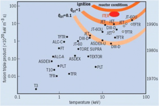
The Lawson criterion is a figure of merit used in nuclear fusion research. It compares the rate of energy being generated by fusion reactions within the fusion fuel to the rate of energy losses to the environment. When the rate of production is higher than the rate of loss, the system will produce net energy. If enough of that energy is captured by the fuel, the system will become self-sustaining and is said to be ignited.
In physics, the Hanbury Brown and Twiss (HBT) effect is any of a variety of correlation and anti-correlation effects in the intensities received by two detectors from a beam of particles. HBT effects can generally be attributed to the wave–particle duality of the beam, and the results of a given experiment depend on whether the beam is composed of fermions or bosons. Devices which use the effect are commonly called intensity interferometers and were originally used in astronomy, although they are also heavily used in the field of quantum optics.
Fluorescence correlation spectroscopy (FCS) is a statistical analysis, via time correlation, of stationary fluctuations of the fluorescence intensity. Its theoretical underpinning originated from L. Onsager's regression hypothesis. The analysis provides kinetic parameters of the physical processes underlying the fluctuations. One of the interesting applications of this is an analysis of the concentration fluctuations of fluorescent particles (molecules) in solution. In this application, the fluorescence emitted from a very tiny space in solution containing a small number of fluorescent particles (molecules) is observed. The fluorescence intensity is fluctuating due to Brownian motion of the particles. In other words, the number of the particles in the sub-space defined by the optical system is randomly changing around the average number. The analysis gives the average number of fluorescent particles and average diffusion time, when the particle is passing through the space. Eventually, both the concentration and size of the particle (molecule) are determined. Both parameters are important in biochemical research, biophysics, and chemistry.
Radiation trapping, imprisonment of resonance radiation, radiative transfer of spectral lines, line transfer or radiation diffusion is a phenomenon in physics whereby radiation may be "trapped" in a system as it is emitted by one atom and absorbed by another.

The stretched exponential function
The theoretical and experimental justification for the Schrödinger equation motivates the discovery of the Schrödinger equation, the equation that describes the dynamics of nonrelativistic particles. The motivation uses photons, which are relativistic particles with dynamics described by Maxwell's equations, as an analogue for all types of particles.

Rotational diffusion is the rotational movement which acts upon any object such as particles, molecules, atoms when present in a fluid, by random changes in their orientations. Whilst the directions and intensities of these changes are statistically random, they do not arise randomly and are instead the result of interactions between particles. One example occurs in colloids, where relatively large insoluble particles are suspended in a greater amount of fluid. The changes in orientation occur from collisions between the particle and the many molecules forming the fluid surrounding the particle, which each transfer kinetic energy to the particle, and as such can be considered random due to the varied speeds and amounts of fluid molecules incident on each individual particle at any given time.
Resonance fluorescence is the process in which a two-level atom system interacts with the quantum electromagnetic field if the field is driven at a frequency near to the natural frequency of the atom.
Fluorescence cross-correlation spectroscopy (FCCS) is a spectroscopic technique that examines the interactions of fluorescent particles of different colours as they randomly diffuse through a microscopic detection volume over time, under steady conditions.
Photon antibunching generally refers to a light field with photons more equally spaced than a coherent laser field, a signature being signals at appropriate detectors which are anticorrelated. More specifically, it can refer to sub-Poissonian photon statistics, that is a photon number distribution for which the variance is less than the mean. A coherent state, as output by a laser far above threshold, has Poissonian statistics yielding random photon spacing; while a thermal light field has super-Poissonian statistics and yields bunched photon spacing. In the thermal (bunched) case, the number of fluctuations is larger than a coherent state; for an antibunched source they are smaller.

In probability theory and directional statistics, a wrapped exponential distribution is a wrapped probability distribution that results from the "wrapping" of the exponential distribution around the unit circle.
In quantum mechanics, magnetic resonance is a resonant effect that can appear when a magnetic dipole is exposed to a static magnetic field and perturbed with another, oscillating electromagnetic field. Due to the static field, the dipole can assume a number of discrete energy eigenstates, depending on the value of its angular momentum (azimuthal) quantum number. The oscillating field can then make the dipole transit between its energy states with a certain probability and at a certain rate. The overall transition probability will depend on the field's frequency and the rate will depend on its amplitude. When the frequency of that field leads to the maximum possible transition probability between two states, a magnetic resonance has been achieved. In that case, the energy of the photons composing the oscillating field matches the energy difference between said states. If the dipole is tickled with a field oscillating far from resonance, it is unlikely to transition. That is analogous to other resonant effects, such as with the forced harmonic oscillator. The periodic transition between the different states is called Rabi cycle and the rate at which that happens is called Rabi frequency. The Rabi frequency should not be confused with the field's own frequency. Since many atomic nuclei species can behave as a magnetic dipole, this resonance technique is the basis of nuclear magnetic resonance, including nuclear magnetic resonance imaging and nuclear magnetic resonance spectroscopy.

The perturbed γ-γ angular correlation, PAC for short or PAC-Spectroscopy, is a method of nuclear solid-state physics with which magnetic and electric fields in crystal structures can be measured. In doing so, electrical field gradients and the Larmor frequency in magnetic fields as well as dynamic effects are determined. With this very sensitive method, which requires only about 10–1000 billion atoms of a radioactive isotope per measurement, material properties in the local structure, phase transitions, magnetism and diffusion can be investigated. The PAC method is related to nuclear magnetic resonance and the Mössbauer effect, but shows no signal attenuation at very high temperatures. Today only the time-differential perturbed angular correlation (TDPAC) is used.


