Difference in differences

Last updated May 03, 2024

Difference in differences (DID^[1] or DD^[2]) is a statistical technique used in econometrics and quantitative research in the social sciences that attempts to mimic an experimental research design using observational study data, by studying the differential effect of a treatment on a 'treatment group' versus a 'control group' in a natural experiment.^[3] It calculates the effect of a treatment (i.e., an explanatory variable or an independent variable) on an outcome (i.e., a response variable or dependent variable) by comparing the average change over time in the outcome variable for the treatment group to the average change over time for the control group. Although it is intended to mitigate the effects of extraneous factors and selection bias, depending on how the treatment group is chosen, this method may still be subject to certain biases (e.g., mean regression, reverse causality and omitted variable bias).

In contrast to a time-series estimate of the treatment effect on subjects (which analyzes differences over time) or a cross-section estimate of the treatment effect (which measures the difference between treatment and control groups), difference in differences uses panel data to measure the differences, between the treatment and control group, of the changes in the outcome variable that occur over time.

General definition

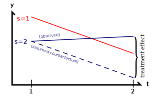
Difference in differences requires data measured from a treatment group and a control group at two or more different time periods, specifically at least one time period before "treatment" and at least one time period after "treatment." In the example pictured, the outcome in the treatment group is represented by the line P and the outcome in the control group is represented by the line S. The outcome (dependent) variable in both groups is measured at time 1, before either group has received the treatment (i.e., the independent or explanatory variable), represented by the points P₁ and S₁. The treatment group then receives or experiences the treatment and both groups are again measured at time 2. Not all of the difference between the treatment and control groups at time 2 (that is, the difference between P₂ and S₂) can be explained as being an effect of the treatment, because the treatment group and control group did not start out at the same point at time 1. DID, therefore, calculates the "normal" difference in the outcome variable between the two groups (the difference that would still exist if neither group experienced the treatment), represented by the dotted line Q. (Notice that the slope from P₁ to Q is the same as the slope from S₁ to S₂.) The treatment effect is the difference between the observed outcome (P₂) and the "normal" outcome (the difference between P₂ and Q).

Formal definition

Consider the model

y_{it}~=~\gamma _{s(i)}+\lambda _{t}+\delta I(\dots )+\varepsilon _{it}

where $y_{it}$ is the dependent variable for individual $i$ and time $t$ , $s(i)$ is the group to which $i$ belongs (i.e. the treatment or the control group), and $I(\dots )$ is short-hand for the dummy variable equal to 1 when the event described in $(\dots )$ is true, and 0 otherwise. In the plot of time versus $Y$ by group, $\gamma _{s}$ is the vertical intercept for the graph for $s$ , and $\lambda _{t}$ is the time trend shared by both groups according to the parallel trend assumption (see Assumptions below). $\delta$ is the treatment effect, and $\varepsilon _{it}$ is the residual term.

Consider the average of the dependent variable and dummy indicators by group and time:

{\begin{aligned}n_{s}&={\text{ number of individuals in group }}s\\{\overline {y}}_{st}&={\frac {1}{n_{s}}}\sum _{i=1}^{n}y_{it}\ I(s(i)~=~s),\\{\overline {\gamma }}_{s}&={\frac {1}{n_{s}}}\sum _{i=1}^{n}\gamma _{s(i)}\ I(s(i)~=~s)~=~\gamma _{s},\\{\overline {\lambda }}_{st}&={\frac {1}{n_{s}}}\sum _{i=1}^{n}\lambda _{t}\ I(s(i)~=~s)~=~\lambda _{t},\\D_{st}&={\frac {1}{n_{s}}}\sum _{i=1}^{n}I(s(i)~=~{\text{ treatment, }}t{\text{ in after period}})\ I(s(i)~=~s)~=~I(s~=~{\text{ treatment, }}t{\text{ in after period}}),\\{\overline {\varepsilon }}_{st}&={\frac {1}{n_{s}}}\sum _{i=1}^{n}\varepsilon _{it}\ I(s(i)~=~s),\end{aligned}}

and suppose for simplicity that $s=1,2$ and $t=1,2$ . Note that $D_{st}$ is not random; it just encodes how the groups and the periods are labeled. Then

{\begin{aligned}&({\overline {y}}_{11}-{\overline {y}}_{12})-({\overline {y}}_{21}-{\overline {y}}_{22})\\[6pt]={}&{\big [}(\gamma _{1}+\lambda _{1}+\delta D_{11}+{\overline {\varepsilon }}_{11})-(\gamma _{1}+\lambda _{2}+\delta D_{12}+{\overline {\varepsilon }}_{12}){\big ]}\\&\qquad {}-{\big [}(\gamma _{2}+\lambda _{1}+\delta D_{21}+{\overline {\varepsilon }}_{21})-(\gamma _{2}+\lambda _{2}+\delta D_{22}+{\overline {\varepsilon }}_{22}){\big ]}\\[6pt]={}&\delta (D_{11}-D_{12})+\delta (D_{22}-D_{21})+{\overline {\varepsilon }}_{11}-{\overline {\varepsilon }}_{12}+{\overline {\varepsilon }}_{22}-{\overline {\varepsilon }}_{21}.\end{aligned}}

The strict exogeneity assumption then implies that

\operatorname {E} \left[({\overline {y}}_{11}-{\overline {y}}_{12})-({\overline {y}}_{21}-{\overline {y}}_{22})\right]~=~\delta (D_{11}-D_{12})+\delta (D_{22}-D_{21}).

Without loss of generality, assume that $s=2$ is the treatment group, and $t=2$ is the after period, then $D_{22}=1$ and $D_{11}=D_{12}=D_{21}=0$ , giving the DID estimator

{\hat {\delta }}~=~({\overline {y}}_{11}-{\overline {y}}_{12})-({\overline {y}}_{21}-{\overline {y}}_{22}),

which can be interpreted as the treatment effect of the treatment indicated by $D_{st}$ . Below it is shown how this estimator can be read as a coefficient in an ordinary least squares regression. The model described in this section is over-parametrized; to remedy that, one of the coefficients for the dummy variables can be set to 0, for example, we may set $\gamma _{1}=0$ .

Assumptions

All the assumptions of the OLS model apply equally to DID. In addition, DID requires a parallel trend assumption. The parallel trend assumption says that $\lambda _{2}-\lambda _{1}$ are the same in both $s=1$ and $s=2$ . Given that the formal definition above accurately represents reality, this assumption automatically holds. However, a model with $\lambda _{st}~:~\lambda _{22}-\lambda _{21}\neq \lambda _{12}-\lambda _{11}$ may well be more realistic. In order to increase the likelihood of the parallel trend assumption holding, a difference-in-differences approach is often combined with matching.^[4] This involves 'Matching' known 'treatment' units with simulated counterfactual 'control' units: characteristically equivalent units which did not receive treatment. By defining the Outcome Variable as a temporal difference (change in observed outcome between pre- and posttreatment periods), and Matching multiple units in a large sample on the basis of similar pre-treatment histories, the resulting ATE (i.e. the ATT: Average Treatment Effect for the Treated) provides a robust difference-in-differences estimate of treatment effects. This serves two statistical purposes: firstly, conditional on pre-treatment covariates, the parallel trends assumption is likely to hold; and secondly, this approach reduces dependence on associated ignorability assumptions necessary for valid inference.

As illustrated to the right, the treatment effect is the difference between the observed value of y and what the value of y would have been with parallel trends, had there been no treatment. The Achilles' heel of DID is when something other than the treatment changes in one group but not the other at the same time as the treatment, implying a violation of the parallel trend assumption.

To guarantee the accuracy of the DID estimate, the composition of individuals of the two groups is assumed to remain unchanged over time. When using a DID model, various issues that may compromise the results, such as autocorrelation ^[5] and Ashenfelter dips, must be considered and dealt with.

Implementation

The DID method can be implemented according to the table below, where the lower right cell is the DID estimator.

$y_{st}$	$s=2$	$s=1$	Difference
$t=2$	$y_{22}$	$y_{12}$	$y_{12}-y_{22}$
$t=1$	$y_{21}$	$y_{11}$	$y_{11}-y_{21}$
Change	$y_{21}-y_{22}$	$y_{11}-y_{12}$	$(y_{11}-y_{21})-(y_{12}-y_{22})$

Running a regression analysis gives the same result. Consider the OLS model

y~=~\beta _{0}+\beta _{1}T+\beta _{2}S+\beta _{3}(T\cdot S)+\varepsilon

where $T$ is a dummy variable for the period, equal to $1$ when $t=2$ , and $S$ is a dummy variable for group membership, equal to $1$ when $s=2$ . The composite variable $(T\cdot S)$ is a dummy variable indicating when $S=T=1$ . Although it is not shown rigorously here, this is a proper parametrization of the model formal definition, furthermore, it turns out that the group and period averages in that section relate to the model parameter estimates as follows

{\begin{aligned}{\hat {\beta }}_{0}&={\widehat {E}}(y\mid T=0,~S=0)\\[8pt]{\hat {\beta }}_{1}&={\widehat {E}}(y\mid T=1,~S=0)-{\widehat {E}}(y\mid T=0,~S=0)\\[8pt]{\hat {\beta }}_{2}&={\widehat {E}}(y\mid T=0,~S=1)-{\widehat {E}}(y\mid T=0,~S=0)\\[8pt]{\hat {\beta }}_{3}&={\big [}{\widehat {E}}(y\mid T=1,~S=1)-{\widehat {E}}(y\mid T=0,~S=1){\big ]}\\&\qquad {}-{\big [}{\widehat {E}}(y\mid T=1,~S=0)-{\widehat {E}}(y\mid T=0,~S=0){\big ]},\end{aligned}}

where ${\widehat {E}}(\dots \mid \dots )$ stands for conditional averages computed on the sample, for example, $T=1$ is the indicator for the after period, $S=0$ is an indicator for the control group. Note that ${\hat {\beta }}_{1}$ is an estimate of the counterfactual rather than the impact of the control group. The control group is often used as a proxy for the counterfactual (see, Synthetic control method for a deeper understanding of this point). Thereby, ${\hat {\beta }}_{1}$ can be interpreted as the impact of both the control group and the intervention's (treatment's) counterfactual. Similarly, ${\hat {\beta }}_{2}$ , due to the parallel trend assumption, is also the same differential between the treatment and control group in $T=1$ . The above descriptions should not be construed to imply the (average) effect of only the control group, for ${\hat {\beta }}_{1}$ , or only the difference of the treatment and control groups in the pre-period, for ${\hat {\beta }}_{2}$ . As in Card and Krueger, below, a first (time) difference of the outcome variable $(\Delta Y_{i}=Y_{i,1}-Y_{i,0})$ eliminates the need for time-trend (i.e., ${\hat {\beta }}_{1}$ ) to form an unbiased estimate of ${\hat {\beta }}_{3}$ , implying that ${\hat {\beta }}_{1}$ is not actually conditional on the treatment or control group.^[6] Consistently, a difference among the treatment and control groups would eliminate the need for treatment differentials (i.e., ${\hat {\beta }}_{2}$ ) to form an unbiased estimate of ${\hat {\beta }}_{3}$ . This nuance is important to understand when the user believes (weak) violations of parallel pre-trend exist or in the case of violations of the appropriate counterfactual approximation assumptions given the existence of non-common shocks or confounding events. To see the relation between this notation and the previous section, consider as above only one observation per time period for each group, then

{\begin{aligned}{\widehat {E}}(y\mid T=1,~S=0)&={\widehat {E}}(y\mid {\text{ after period, control}})\\[3pt]\\&={\frac {{\widehat {E}}(y\ I({\text{ after period, control}}))}{{\widehat {P}}({\text{ after period, control}})}}\\[3pt]\\&={\frac {\sum _{i=1}^{n}y_{i,{\text{after}}}I(i{\text{ in control}})}{n_{\text{control}}}}={\overline {y}}_{\text{control, after}}\\[3pt]\\&={\overline {y}}_{\text{12}}\end{aligned}}

and so on for other values of $T$ and $S$ , which is equivalent to

{\hat {\beta }}_{3}~=~(y_{11}-y_{21})-(y_{12}-y_{22}).

But this is the expression for the treatment effect that was given in the formal definition and in the above table.

Card and Krueger (1994) example

The Card and Krueger article on minimum wage in New Jersey, published in 1994,^[6] is considered one of the most famous DID studies; Card was later awarded the 2021 Nobel Memorial Prize in Economic Sciences in part for this and related work. Card and Krueger compared employment in the fast food sector in New Jersey and in Pennsylvania, in February 1992 and in November 1992, after New Jersey's minimum wage rose from $4.25 to $5.05 in April 1992. Observing a change in employment in New Jersey only, before and after the treatment, would fail to control for omitted variables such as weather and macroeconomic conditions of the region. By including Pennsylvania as a control in a difference-in-differences model, any bias caused by variables common to New Jersey and Pennsylvania is implicitly controlled for, even when these variables are unobserved. Assuming that New Jersey and Pennsylvania have parallel trends over time, Pennsylvania's change in employment can be interpreted as the change New Jersey would have experienced, had they not increased the minimum wage, and vice versa. The evidence suggested that the increased minimum wage did not induce a decrease in employment in New Jersey, contrary to what some economic theory would suggest. The table below shows Card & Krueger's estimates of the treatment effect on employment, measured as FTEs (or full-time equivalents). Card and Krueger estimate that the $0.80 minimum wage increase in New Jersey led to a 2.75 FTE increase in employment.

	New Jersey	Pennsylvania	Difference
February	20.44	23.33	−2.89
November	21.03	21.17	−0.14
Change	0.59	−2.16	2.75

A software example application of this research is found on the Stata's command -diff- ^[7] authored by Juan Miguel Villa.

Related Research Articles

In probability theory and statistics, the exponential distribution or negative exponential distribution is the probability distribution of the distance between events in a Poisson point process, i.e., a process in which events occur continuously and independently at a constant average rate; the distance parameter could be any meaningful mono-dimensional measure of the process, such as time between production errors, or length along a roll of fabric in the weaving manufacturing process. It is a particular case of the gamma distribution. It is the continuous analogue of the geometric distribution, and it has the key property of being memoryless. In addition to being used for the analysis of Poisson point processes it is found in various other contexts.

In statistics, the Gauss–Markov theorem states that the ordinary least squares (OLS) estimator has the lowest sampling variance within the class of linear unbiased estimators, if the errors in the linear regression model are uncorrelated, have equal variances and expectation value of zero. The errors do not need to be normal for the theorem to apply, nor do they need to be independent and identically distributed.

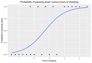
In statistics, the logistic model is a statistical model that models the log-odds of an event as a linear combination of one or more independent variables. In regression analysis, logistic regression is estimating the parameters of a logistic model. Formally, in binary logistic regression there is a single binary dependent variable, coded by an indicator variable, where the two values are labeled "0" and "1", while the independent variables can each be a binary variable or a continuous variable. The corresponding probability of the value labeled "1" can vary between 0 and 1, hence the labeling; the function that converts log-odds to probability is the logistic function, hence the name. The unit of measurement for the log-odds scale is called a logit, from logistic unit, hence the alternative names. See § Background and § Definition for formal mathematics, and § Example for a worked example.

In vector calculus, Green's theorem relates a line integral around a simple closed curve $C$ to a double integral over the plane region $D$ bounded by $C$ . It is the two-dimensional special case of Stokes' theorem.

In statistics, Deming regression, named after W. Edwards Deming, is an errors-in-variables model that tries to find the line of best fit for a two-dimensional data set. It differs from the simple linear regression in that it accounts for errors in observations on both the x- and the y- axis. It is a special case of total least squares, which allows for any number of predictors and a more complicated error structure.

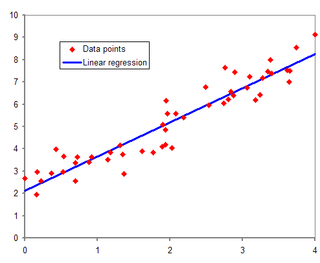
In statistical modeling, regression analysis is a set of statistical processes for estimating the relationships between a dependent variable and one or more independent variables. The most common form of regression analysis is linear regression, in which one finds the line that most closely fits the data according to a specific mathematical criterion. For example, the method of ordinary least squares computes the unique line that minimizes the sum of squared differences between the true data and that line. For specific mathematical reasons, this allows the researcher to estimate the conditional expectation of the dependent variable when the independent variables take on a given set of values. Less common forms of regression use slightly different procedures to estimate alternative location parameters or estimate the conditional expectation across a broader collection of non-linear models.

In statistics, the theory of minimum norm quadratic unbiased estimation (MINQUE) was developed by C. R. Rao. MINQUE is a theory alongside other estimation methods in estimation theory, such as the method of moments or maximum likelihood estimation. Similar to the theory of best linear unbiased estimation, MINQUE is specifically concerned with linear regression models. The method was originally conceived to estimate heteroscedastic error variance in multiple linear regression. MINQUE estimators also provide an alternative to maximum likelihood estimators or restricted maximum likelihood estimators for variance components in mixed effects models. MINQUE estimators are quadratic forms of the response variable and are used to estimate a linear function of the variances.

In statistics, ordinary least squares (OLS) is a type of linear least squares method for choosing the unknown parameters in a linear regression model by the principle of least squares: minimizing the sum of the squares of the differences between the observed dependent variable in the input dataset and the output of the (linear) function of the independent variable.

In statistics, simple linear regression (SLR) is a linear regression model with a single explanatory variable. That is, it concerns two-dimensional sample points with one independent variable and one dependent variable and finds a linear function that, as accurately as possible, predicts the dependent variable values as a function of the independent variable. The adjective simple refers to the fact that the outcome variable is related to a single predictor.

In statistics, a fixed effects model is a statistical model in which the model parameters are fixed or non-random quantities. This is in contrast to random effects models and mixed models in which all or some of the model parameters are random variables. In many applications including econometrics and biostatistics a fixed effects model refers to a regression model in which the group means are fixed (non-random) as opposed to a random effects model in which the group means are a random sample from a population. Generally, data can be grouped according to several observed factors. The group means could be modeled as fixed or random effects for each grouping. In a fixed effects model each group mean is a group-specific fixed quantity.

In statistics, generalized least squares (GLS) is a method used to estimate the unknown parameters in a linear regression model. It is used when there is a non-zero amount of correlation between the residuals in the regression model. GLS is employed to improve statistical efficiency and reduce the risk of drawing erroneous inferences, as compared to conventional least squares and weighted least squares methods. It was first described by Alexander Aitken in 1935.

The Newman–Penrose (NP) formalism is a set of notation developed by Ezra T. Newman and Roger Penrose for general relativity (GR). Their notation is an effort to treat general relativity in terms of spinor notation, which introduces complex forms of the usual variables used in GR. The NP formalism is itself a special case of the tetrad formalism, where the tensors of the theory are projected onto a complete vector basis at each point in spacetime. Usually this vector basis is chosen to reflect some symmetry of the spacetime, leading to simplified expressions for physical observables. In the case of the NP formalism, the vector basis chosen is a null tetrad: a set of four null vectors—two real, and a complex-conjugate pair. The two real members often asymptotically point radially inward and radially outward, and the formalism is well adapted to treatment of the propagation of radiation in curved spacetime. The Weyl scalars, derived from the Weyl tensor, are often used. In particular, it can be shown that one of these scalars— $in the appropriate frame—encodes the outgoing gravitational radiation of an asymptotically flat system.$

In the Newman–Penrose (NP) formalism of general relativity, Weyl scalars refer to a set of five complex scalars $which encode the ten independent components of the Weyl tensor of a four-dimensional spacetime.$

Bayesian linear regression is a type of conditional modeling in which the mean of one variable is described by a linear combination of other variables, with the goal of obtaining the posterior probability of the regression coefficients and ultimately allowing the out-of-sample prediction of the regressandconditional on observed values of the regressors. The simplest and most widely used version of this model is the normal linear model, in which $given is distributed Gaussian. In this model, and under a particular choice of prior probabilities for the parameters—so-called conjugate priors—the posterior can be found analytically. With more arbitrarily chosen priors, the posteriors generally have to be approximated.$

In statistics, principal component regression (PCR) is a regression analysis technique that is based on principal component analysis (PCA). More specifically, PCR is used for estimating the unknown regression coefficients in a standard linear regression model.

In statistics, a sum of squares due to lack of fit, or more tersely a lack-of-fit sum of squares, is one of the components of a partition of the sum of squares of residuals in an analysis of variance, used in the numerator in an F-test of the null hypothesis that says that a proposed model fits well. The other component is the pure-error sum of squares.

The purpose of this page is to provide supplementary materials for the ordinary least squares article, reducing the load of the main article with mathematics and improving its accessibility, while at the same time retaining the completeness of exposition.

In the Newman–Penrose (NP) formalism of general relativity, independent components of the Ricci tensors of a four-dimensional spacetime are encoded into seven Ricci scalars which consist of three real scalars $, three complex scalars and the NP curvature scalar . Physically, Ricci-NP scalars are related with the energy-momentum distribution of the spacetime due to Einstein's field equation.$

Symmetries in quantum mechanics describe features of spacetime and particles which are unchanged under some transformation, in the context of quantum mechanics, relativistic quantum mechanics and quantum field theory, and with applications in the mathematical formulation of the standard model and condensed matter physics. In general, symmetry in physics, invariance, and conservation laws, are fundamentally important constraints for formulating physical theories and models. In practice, they are powerful methods for solving problems and predicting what can happen. While conservation laws do not always give the answer to the problem directly, they form the correct constraints and the first steps to solving a multitude of problems. In application, understanding symmetries can also provide insights on the eigenstates that can be expected. For example, the existence of degenerate states can be inferred by the presence of non commuting symmetry operators or that the non degenerate states are also eigenvectors of symmetry operators.

In set theory and logic, Buchholz's ID hierarchy is a hierarchy of subsystems of first-order arithmetic. The systems/theories $are referred to as "the formal theories of ν-times iterated inductive definitions". ID ν extends PA by ν iterated least fixed points of monotone operators.$

References

↑ Abadie, A. (2005). "Semiparametric difference-in-differences estimators". Review of Economic Studies . 72 (1): 1–19. CiteSeerX 10.1.1.470.1475 . doi:10.1111/0034-6527.00321. S2CID 8801460.
↑ Bertrand, M.; Duflo, E.; Mullainathan, S. (2004). "How Much Should We Trust Differences-in-Differences Estimates?" (PDF). Quarterly Journal of Economics . 119 (1): 249–275. doi:10.1162/003355304772839588. S2CID 470667.
↑ Angrist, J. D.; Pischke, J. S. (2008). Mostly Harmless Econometrics: An Empiricist's Companion. Princeton University Press. pp. 227–243. ISBN 978-0-691-12034-8.
↑ Basu, Pallavi; Small, Dylan (2020). "Constructing a More Closely Matched Control Group in a Difference-in-Differences Analysis: Its Effect on History Interacting with Group Bias". Observational Studies . 6: 103–130. doi:10.1353/obs.2020.0011. S2CID 221702893.
↑ Bertrand, Marianne; Duflo, Esther; Mullainathan, Sendhil (2004). "How Much Should We Trust Differences-In-Differences Estimates?" (PDF). Quarterly Journal of Economics . 119 (1): 249–275. doi:10.1162/003355304772839588. S2CID 470667.
1 2 Card, David; Krueger, Alan B. (1994). "Minimum Wages and Employment: A Case Study of the Fast-Food Industry in New Jersey and Pennsylvania". American Economic Review . 84 (4): 772–793. JSTOR 2118030.
↑ Villa, Juan M. (2016). "diff: Simplifying the estimation of difference-in-differences treatment effects". The Stata Journal. 16 (1): 52–71. doi: 10.1177/1536867X1601600108 . S2CID 124464636.

External links

Difference in Difference Estimation, Healthcare Economist website

This page is based on this Wikipedia article
Text is available under the CC BY-SA 4.0 license; additional terms may apply.
Images, videos and audio are available under their respective licenses.

[1] Abadie, A. (2005). "Semiparametric difference-in-differences estimators". Review of Economic Studies . 72 (1): 1–19. CiteSeerX 10.1.1.470.1475 . doi:10.1111/0034-6527.00321. S2CID 8801460.

[Bertrand-2] Bertrand, M.; Duflo, E.; Mullainathan, S. (2004). "How Much Should We Trust Differences-in-Differences Estimates?" (PDF). Quarterly Journal of Economics . 119 (1): 249–275. doi:10.1162/003355304772839588. S2CID 470667.

[3] Angrist, J. D.; Pischke, J. S. (2008). Mostly Harmless Econometrics: An Empiricist's Companion. Princeton University Press. pp. 227–243. ISBN 978-0-691-12034-8.

[4] Basu, Pallavi; Small, Dylan (2020). "Constructing a More Closely Matched Control Group in a Difference-in-Differences Analysis: Its Effect on History Interacting with Group Bias". Observational Studies . 6: 103–130. doi:10.1353/obs.2020.0011. S2CID 221702893.

[5] Bertrand, Marianne; Duflo, Esther; Mullainathan, Sendhil (2004). "How Much Should We Trust Differences-In-Differences Estimates?" (PDF). Quarterly Journal of Economics . 119 (1): 249–275. doi:10.1162/003355304772839588. S2CID 470667.

[David-6] 1 2 Card, David; Krueger, Alan B. (1994). "Minimum Wages and Employment: A Case Study of the Fast-Food Industry in New Jersey and Pennsylvania". American Economic Review . 84 (4): 772–793. JSTOR 2118030.

[StataDiff-7] Villa, Juan M. (2016). "diff: Simplifying the estimation of difference-in-differences treatment effects". The Stata Journal. 16 (1): 52–71. doi: 10.1177/1536867X1601600108 . S2CID 124464636.

[1]

[2]

[3]

[4]

[5]

[6]

[7]