In mathematics, and more specifically in linear algebra, a linear map is a mapping between two vector spaces that preserves the operations of vector addition and scalar multiplication. The same names and the same definition are also used for the more general case of modules over a ring; see Module homomorphism.

In mathematics, the linear span (also called the linear hull or just span) of a set S of vectors (from a vector space), denoted span(S), is defined as the set of all linear combinations of the vectors in S. For example, two linearly independent vectors span a plane. The linear span can be characterized either as the intersection of all linear subspaces that contain S, or as the smallest subspace containing S. The linear span of a set of vectors is therefore a vector space itself. Spans can be generalized to matroids and modules.
A weight function is a mathematical device used when performing a sum, integral, or average to give some elements more "weight" or influence on the result than other elements in the same set. The result of this application of a weight function is a weighted sum or weighted average. Weight functions occur frequently in statistics and analysis, and are closely related to the concept of a measure. Weight functions can be employed in both discrete and continuous settings. They can be used to construct systems of calculus called "weighted calculus" and "meta-calculus".

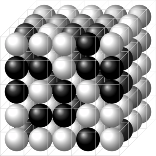
In mathematical physics, a lattice model is a mathematical model of a physical system that is defined on a lattice, as opposed to a continuum, such as the continuum of space or spacetime. Lattice models originally occurred in the context of condensed matter physics, where the atoms of a crystal automatically form a lattice. Currently, lattice models are quite popular in theoretical physics, for many reasons. Some models are exactly solvable, and thus offer insight into physics beyond what can be learned from perturbation theory. Lattice models are also ideal for study by the methods of computational physics, as the discretization of any continuum model automatically turns it into a lattice model. The exact solution to many of these models includes the presence of solitons. Techniques for solving these include the inverse scattering transform and the method of Lax pairs, the Yang–Baxter equation and quantum groups. The solution of these models has given insights into the nature of phase transitions, magnetization and scaling behaviour, as well as insights into the nature of quantum field theory. Physical lattice models frequently occur as an approximation to a continuum theory, either to give an ultraviolet cutoff to the theory to prevent divergences or to perform numerical computations. An example of a continuum theory that is widely studied by lattice models is the QCD lattice model, a discretization of quantum chromodynamics. However, digital physics considers nature fundamentally discrete at the Planck scale, which imposes upper limit to the density of information, aka Holographic principle. More generally, lattice gauge theory and lattice field theory are areas of study. Lattice models are also used to simulate the structure and dynamics of polymers.

In mathematics, an affine space is a geometric structure that generalizes some of the properties of Euclidean spaces in such a way that these are independent of the concepts of distance and measure of angles, keeping only the properties related to parallelism and ratio of lengths for parallel line segments.

In mathematics and theoretical physics, the term quantum group denotes one of a few different kinds of noncommutative algebras with additional structure. These include Drinfeld–Jimbo type quantum groups, compact matrix quantum groups, and bicrossproduct quantum groups. Despite their name, they do not themselves have a natural group structure, though they are in some sense 'close' to a group.
In probability theory, a compound Poisson distribution is the probability distribution of the sum of a number of independent identically-distributed random variables, where the number of terms to be added is itself a Poisson-distributed variable. The result can be either a continuous or a discrete distribution.
In statistics, multicollinearity is a phenomenon in which one predictor variable in a multiple regression model can be linearly predicted from the others with a substantial degree of accuracy. In this situation, the coefficient estimates of the multiple regression may change erratically in response to small changes in the model or the data. Multicollinearity does not reduce the predictive power or reliability of the model as a whole, at least within the sample data set; it only affects calculations regarding individual predictors. That is, a multivariable regression model with collinear predictors can indicate how well the entire bundle of predictors predicts the outcome variable, but it may not give valid results about any individual predictor, or about which predictors are redundant with respect to others.
In linear algebra, an eigenvector or characteristic vector of a linear transformation is a nonzero vector that changes at most by a scalar factor when that linear transformation is applied to it. The corresponding eigenvalue, often denoted by , is the factor by which the eigenvector is scaled.
In statistics, Poisson regression is a generalized linear model form of regression analysis used to model count data and contingency tables. Poisson regression assumes the response variable Y has a Poisson distribution, and assumes the logarithm of its expected value can be modeled by a linear combination of unknown parameters. A Poisson regression model is sometimes known as a log-linear model, especially when used to model contingency tables.
Verma modules, named after Daya-Nand Verma, are objects in the representation theory of Lie algebras, a branch of mathematics.
Linear Programming Boosting (LPBoost) is a supervised classifier from the boosting family of classifiers. LPBoost maximizes a margin between training samples of different classes and hence also belongs to the class of margin-maximizing supervised classification algorithms. Consider a classification function
In statistics, principal component regression (PCR) is a regression analysis technique that is based on principal component analysis (PCA). More specifically, PCR is used for estimating the unknown regression coefficients in a standard linear regression model.
In applied mathematics, the Atkinson–Mingarelli theorem, named after Frederick Valentine Atkinson and A. B. Mingarelli, concerns eigenvalues of certain Sturm–Liouville differential operators.
Log-linear analysis is a technique used in statistics to examine the relationship between more than two categorical variables. The technique is used for both hypothesis testing and model building. In both these uses, models are tested to find the most parsimonious model that best accounts for the variance in the observed frequencies.

In probability, statistics and related fields, a Poisson point process is a type of random mathematical object that consists of points randomly located on a mathematical space with the essential feature that the points occur independently of one another. The Poisson point process is often called simply the Poisson process, but it is also called a Poisson random measure, Poisson random point field or Poisson point field. This point process has convenient mathematical properties, which has led to its being frequently defined in Euclidean space and used as a mathematical model for seemingly random processes in numerous disciplines such as astronomy, biology, ecology, geology, seismology, physics, economics, image processing, and telecommunications.
Structured sparsity regularization is a class of methods, and an area of research in statistical learning theory, that extend and generalize sparsity regularization learning methods. Both sparsity and structured sparsity regularization methods seek to exploit the assumption that the output variable to be learned can be described by a reduced number of variables in the input space . Sparsity regularization methods focus on selecting the input variables that best describe the output. Structured sparsity regularization methods generalize and extend sparsity regularization methods, by allowing for optimal selection over structures like groups or networks of input variables in .

In mathematics, the representation theory of semisimple Lie algebras is one of the crowning achievements of the theory of Lie groups and Lie algebras. The theory was worked out mainly by E. Cartan and H. Weyl and because of that, the theory is also known as the Cartan–Weyl theory. The theory gives the structural description and classification of a finite-dimensional representation of a semisimple Lie algebra ; in particular, it gives a way to parametrize irreducible finite-dimensional representations of a semisimple Lie algebra, the result known as the theorem of the highest weight.

In probability theory, a birth process or a pure birth process is a special case of a continuous-time Markov process and a generalisation of a Poisson process. It defines a continuous process which takes values in the natural numbers and can only increase by one or remain unchanged. This is a type of birth–death process with no deaths. The rate at which births occur is given by an exponential random variable whose parameter depends only on the current value of the process
Tau functions are an important ingredient in the modern theory of integrable systems, and have numerous applications in a variety of other domains. They were originally introduced by Ryogo Hirota in his direct method approach to soliton equations, based on expressing them in an equivalent bilinear form. The term Tau function, or -function, was first used systematically by Mikio Sato and his students in the specific context of the Kadomtsev–Petviashvili equation and related integrable hierarchies. It is a central ingredient in the theory of solitons. Tau functions also appear as matrix model partition functions in the spectral theory of Random Matrices, and may also serve as generating functions, in the sense of combinatorics and enumerative geometry, especially in relation to moduli spaces of Riemann surfaces, and enumeration of branched coverings, or so-called Hurwitz numbers.


