Dynamic perfect hashing

Last updated

In computer science, dynamic perfect hashing is a programming technique for resolving collisions in a hash table data structure. [1] [2] [3] While more memory-intensive than its hash table counterparts,[ citation needed ] this technique is useful for situations where fast queries, insertions, and deletions must be made on a large set of elements.

Contents

Details

Static case

FKS Scheme

The problem of optimal static hashing was first solved in general by Fredman, Komlós and Szemerédi. [4] In their 1984 paper, [1] they detail a two-tiered hash table scheme in which each bucket of the (first-level) hash table corresponds to a separate second-level hash table. Keys are hashed twice—the first hash value maps to a certain bucket in the first-level hash table; the second hash value gives the position of that entry in that bucket's second-level hash table. The second-level table is guaranteed to be collision-free (i.e. perfect hashing) upon construction. Consequently, the look-up cost is guaranteed to be O(1) in the worst-case. [2]

In the static case, we are given a set with a total of x entries, each one with a unique key, ahead of time. Fredman, Komlós and Szemerédi pick a first-level hash table with size buckets. [2]

To construct, x entries are separated into s buckets by the top-level hashing function, where . Then for each bucket with k entries, a second-level table is allocated with slots, and its hash function is selected at random from a universal hash function set so that it is collision-free (i.e. a perfect hash function) and stored alongside the hash table. If the hash function randomly selected creates a table with collisions, a new hash function is randomly selected until a collision-free table can be guaranteed. Finally, with the collision-free hash, the k entries are hashed into the second-level table.

The quadratic size of the space ensures that randomly creating a table with collisions is infrequent and independent of the size of k, providing linear amortized construction time. Although each second-level table requires quadratic space, if the keys inserted into the first-level hash table are uniformly distributed, the structure as a whole occupies expected space, since bucket sizes are small with high probability. [1]

The first-level hash function is specifically chosen so that, for the specific set of x unique key values, the total space T used by all the second-level hash tables has expected space, and more specifically . Fredman, Komlós and Szemerédi showed that given a universal hashing family of hash functions, at least half of those functions have that property. [2]

Dynamic case

Dietzfelbinger et al. present a dynamic dictionary algorithm that, when a set of n items is incrementally added to the dictionary, membership queries always run in constant time and therefore worst-case time, the total storage required is (linear), and expected amortized insertion and deletion time (amortized constant time).

In the dynamic case, when a key is inserted into the hash table, if its entry in its respective subtable is occupied, then a collision is said to occur and the subtable is rebuilt based on its new total entry count and randomly selected hash function. Because the load factor of the second-level table is kept low , rebuilding is infrequent, and the amortized expected cost of insertions is . [2] Similarly, the amortized expected cost of deletions is . [2]

Additionally, the ultimate sizes of the top-level table or any of the subtables is unknowable in the dynamic case. One method for maintaining expected space of the table is to prompt a full reconstruction when a sufficient number of insertions and deletions have occurred. By results due to Dietzfelbinger et al., [2] as long as the total number of insertions or deletions exceeds the number of elements at the time of last construction, the amortized expected cost of insertion and deletion remain with full rehashing taken into consideration.

The implementation of dynamic perfect hashing by Dietzfelbinger et al. uses these concepts, as well as lazy deletion, and is shown in pseudocode below.

Pseudocode implementation

Locate

function Locate(x) isj := h(x)     if (position hj(x) of subtable Tj contains x (not deleted))         return (x is in S)     end ifelsereturn (x is not in S)     end elseend

Insert

During the insertion of a new entry x at j, the global operations counter, count, is incremented.

If x exists at j, but is marked as deleted, then the mark is removed.

If x exists at j or at the subtable Tj, and is not marked as deleted, then a collision is said to occur and the jth bucket's second-level table Tj is rebuilt with a different randomly selected hash function hj.

function Insert(x) iscount = count + 1;     if (count > M)          FullRehash(x);     end ifelsej = h(x);         if (Position hj(x) of subtable Tj contains x)             if (x is marked deleted)                  remove the delete marker;             end ifend ifelsebj = bj + 1;             if (bj <= mj)                  if position hj(x) of Tj is empty                      store x in position hj(x) of Tj;                 end ifelse                     Put all unmarked elements of Tj in list Lj;                     Append x to list Lj;                     bj = length of Lj;                     repeathj = randomly chosen function in Hsj;                     untilhj is injective on the elements of Lj;                     for all y on list Lj                         store y in position hj(y) of Tj;                     end forend elseend ifelsemj = 2 * max{1, mj};                 sj = 2 * mj * (mj - 1);                 if the sum total of all sj ≤ 32 * M2 / s(M) + 4 * M                      Allocate sj cells for Tj;                     Put all unmarked elements of Tj in list Lj;                     Append x to list Lj;                     bj = length of Lj;                     repeathj = randomly chosen function in Hsj;                     untilhj is injective on the elements of Lj;                     for all y on list Lj                         store y in position hj(y) of Tj;                     end forend ifelse                     FullRehash(x);                 end elseend elseend elseend elseend

Delete

Deletion of x simply flags x as deleted without removal and increments count. In the case of both insertions and deletions, if count reaches a threshold M the entire table is rebuilt, where M is some constant multiple of the size of S at the start of a new phase. Here phase refers to the time between full rebuilds. Note that here the -1 in "Delete(x)" is a representation of an element which is not in the set of all possible elements U.

function Delete(x) iscount = count + 1;     j = h(x);     if position hj(x) of subtable Tj contains x         mark x as deleted;     end ifelsereturn (x is not a member of S);     end elseif (count >= M)         FullRehash(-1);     end ifend

Full rebuild

A full rebuild of the table of S first starts by removing all elements marked as deleted and then setting the next threshold value M to some constant multiple of the size of S. A hash function, which partitions S into s(M) subsets, where the size of subset j is sj, is repeatedly randomly chosen until:

Finally, for each subtable Tj a hash function hj is repeatedly randomly chosen from Hsj until hj is injective on the elements of Tj. The expected time for a full rebuild of the table of S with size n is O(n). [2]

function FullRehash(x) is     Put all unmarked elements of T in list L;     if (x is in U)          append x to L;     end ifcount = length of list L;     M = (1 + c) * max{count, 4};     repeat          h = randomly chosen function in Hs(M);         for all j < s(M)              form a list Lj for h(x) = j;             bj = length of Lj;              mj = 2 * bj;              sj = 2 * mj * (mj - 1);         end foruntil the sum total of all sj ≤ 32 * M2 / s(M) + 4 * Mfor all j < s(M)          Allocate space sj for subtable Tj;         repeathj = randomly chosen function in Hsj;         untilhj is injective on the elements of list Lj;     end forfor all x on list Lj          store x in position hj(x) of Tj;     end forend

See also

Related Research Articles

<span class="mw-page-title-main">AVL tree</span> Self-balancing binary search tree

In computer science, an AVL tree is a self-balancing binary search tree. It was the first such data structure to be invented. In an AVL tree, the heights of the two child subtrees of any node differ by at most one; if at any time they differ by more than one, rebalancing is done to restore this property. Lookup, insertion, and deletion all take O(log n) time in both the average and worst cases, where is the number of nodes in the tree prior to the operation. Insertions and deletions may require the tree to be rebalanced by one or more tree rotations.

<span class="mw-page-title-main">Hash function</span> Mapping arbitrary data to fixed-size values

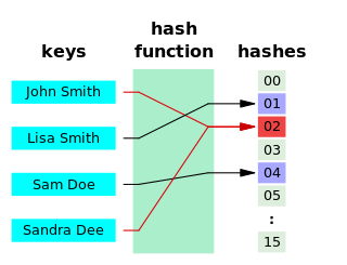
A hash function is any function that can be used to map data of arbitrary size to fixed-size values, though there are some hash functions that support variable length output. The values returned by a hash function are called hash values, hash codes, digests, or simply hashes. The values are usually used to index a fixed-size table called a hash table. Use of a hash function to index a hash table is called hashing or scatter storage addressing.

<span class="mw-page-title-main">Hash table</span> Associative array for storing key-value pairs

In computing, a hash table, also known as hash map, is a data structure that implements an associative array or dictionary. It is an abstract data type that maps keys to values. A hash table uses a hash function to compute an index, also called a hash code, into an array of buckets or slots, from which the desired value can be found. During lookup, the key is hashed and the resulting hash indicates where the corresponding value is stored.

In computer science, an associative array, map, symbol table, or dictionary is an abstract data type that stores a collection of pairs, such that each possible key appears at most once in the collection. In mathematical terms, an associative array is a function with finite domain. It supports 'lookup', 'remove', and 'insert' operations.

<span class="mw-page-title-main">Treap</span>

In computer science, the treap and the randomized binary search tree are two closely related forms of binary search tree data structures that maintain a dynamic set of ordered keys and allow binary searches among the keys. After any sequence of insertions and deletions of keys, the shape of the tree is a random variable with the same probability distribution as a random binary tree; in particular, with high probability its height is proportional to the logarithm of the number of keys, so that each search, insertion, or deletion operation takes logarithmic time to perform.

<span class="mw-page-title-main">Perfect hash function</span> Hash function without any collisions

In computer science, a perfect hash functionh for a set S is a hash function that maps distinct elements in S to a set of m integers, with no collisions. In mathematical terms, it is an injective function.

In information theory, linguistics, and computer science, the Levenshtein distance is a string metric for measuring the difference between two sequences. Informally, the Levenshtein distance between two words is the minimum number of single-character edits required to change one word into the other. It is named after the Soviet mathematician Vladimir Levenshtein, who considered this distance in 1965.

A Bloom filter is a space-efficient probabilistic data structure, conceived by Burton Howard Bloom in 1970, that is used to test whether an element is a member of a set. False positive matches are possible, but false negatives are not – in other words, a query returns either "possibly in set" or "definitely not in set". Elements can be added to the set, but not removed ; the more items added, the larger the probability of false positives.

In computing, a persistent data structure or not ephemeral data structure is a data structure that always preserves the previous version of itself when it is modified. Such data structures are effectively immutable, as their operations do not (visibly) update the structure in-place, but instead always yield a new updated structure. The term was introduced in Driscoll, Sarnak, Sleator, and Tarjans' 1986 article.

In computer science, a scapegoat tree is a self-balancing binary search tree, invented by Arne Andersson in 1989 and again by Igal Galperin and Ronald L. Rivest in 1993. It provides worst-case lookup time and amortized insertion and deletion time.

<span class="mw-page-title-main">Linear probing</span> Computer programming method for hashing

Linear probing is a scheme in computer programming for resolving collisions in hash tables, data structures for maintaining a collection of key–value pairs and looking up the value associated with a given key. It was invented in 1954 by Gene Amdahl, Elaine M. McGraw, and Arthur Samuel and first analyzed in 1963 by Donald Knuth.

<span class="mw-page-title-main">Coalesced hashing</span>

Coalesced hashing, also called coalesced chaining, is a strategy of collision resolution in a hash table that forms a hybrid of separate chaining and open addressing.

<span class="mw-page-title-main">Cuckoo hashing</span> Data structure hashing scheme

Cuckoo hashing is a scheme in computer programming for resolving hash collisions of values of hash functions in a table, with worst-case constant lookup time. The name derives from the behavior of some species of cuckoo, where the cuckoo chick pushes the other eggs or young out of the nest when it hatches in a variation of the behavior referred to as brood parasitism; analogously, inserting a new key into a cuckoo hashing table may push an older key to a different location in the table.

In mathematics and computing, universal hashing refers to selecting a hash function at random from a family of hash functions with a certain mathematical property. This guarantees a low number of collisions in expectation, even if the data is chosen by an adversary. Many universal families are known, and their evaluation is often very efficient. Universal hashing has numerous uses in computer science, for example in implementations of hash tables, randomized algorithms, and cryptography.

2-choice hashing, also known as 2-choice chaining, is "a variant of a hash table in which keys are added by hashing with two hash functions. The key is put in the array position with the fewer (colliding) keys. Some collision resolution scheme is needed, unless keys are kept in buckets. The average-case cost of a successful search is , where is the number of keys and is the size of the array. The most collisions is with high probability."

Database tables and indexes may be stored on disk in one of a number of forms, including ordered/unordered flat files, ISAM, heap files, hash buckets, or B+ trees. Each form has its own particular advantages and disadvantages. The most commonly used forms are B-trees and ISAM. Such forms or structures are one aspect of the overall schema used by a database engine to store information.

<span class="mw-page-title-main">Queap</span>

In computer science, a queap is a priority queue data structure. The data structure allows insertions and deletions of arbitrary elements, as well as retrieval of the highest-priority element. Each deletion takes amortized time logarithmic in the number of items that have been in the structure for a longer time than the removed item. Insertions take constant amortized time.

In computer science, a family of hash functions is said to be k-independent, k-wise independent or k-universal if selecting a function at random from the family guarantees that the hash codes of any designated k keys are independent random variables. Such families allow good average case performance in randomized algorithms or data structures, even if the input data is chosen by an adversary. The trade-offs between the degree of independence and the efficiency of evaluating the hash function are well studied, and many k-independent families have been proposed.

In computer science, the order-maintenance problem involves maintaining a totally ordered set supporting the following operations:

Static Hashing is another form of the hashing problem which allows users to perform lookups on a finalized dictionary set.

References

  1. 1 2 3 Fredman, M. L., Komlós, J., and Szemerédi, E. 1984. Storing a Sparse Table with 0(1) Worst Case Access Time. J. ACM 31, 3 (Jun. 1984), 538-544 http://portal.acm.org/citation.cfm?id=1884#
  2. 1 2 3 4 5 6 7 8 Dietzfelbinger, M., Karlin, A., Mehlhorn, K., Meyer auf der Heide, F., Rohnert, H., and Tarjan, R. E. 1994. "Dynamic Perfect Hashing: Upper and Lower Bounds" Archived 2016-03-04 at the Wayback Machine . SIAM J. Comput. 23, 4 (Aug. 1994), 738-761. http://portal.acm.org/citation.cfm?id=182370 doi : 10.1137/S0097539791194094
  3. Erik Demaine, Jeff Lind. 6.897: Advanced Data Structures. MIT Computer Science and Artificial Intelligence Laboratory. Spring 2003.
  4. Yap, Chee. "Universal Construction for the FKS Scheme". New York University. New York University. Retrieved 15 February 2015.[ permanent dead link ]