In mathematics, the determinant is a scalar value that is a certain function of the entries of a square matrix. The determinant of a matrix A is commonly denoted det(A), det A, or |A|. Its value characterizes some properties of the matrix and the linear map represented, on a given basis, by the matrix. In particular, the determinant is nonzero if and only if the matrix is invertible and the corresponding linear map is an isomorphism. The determinant of a product of matrices is the product of their determinants.

In mathematics, Gaussian elimination, also known as row reduction, is an algorithm for solving systems of linear equations. It consists of a sequence of row-wise operations performed on the corresponding matrix of coefficients. This method can also be used to compute the rank of a matrix, the determinant of a square matrix, and the inverse of an invertible matrix. The method is named after Carl Friedrich Gauss (1777–1855). To perform row reduction on a matrix, one uses a sequence of elementary row operations to modify the matrix until the lower left-hand corner of the matrix is filled with zeros, as much as possible. There are three types of elementary row operations:
In linear algebra, the identity matrix of size is the square matrix with ones on the main diagonal and zeros elsewhere. It has unique properties, for example when the identity matrix represents a geometric transformation, the object remains unchanged by the transformation. In other contexts, it is analogous to multiplying by the number 1.
In linear algebra, an orthogonal matrix, or orthonormal matrix, is a real square matrix whose columns and rows are orthonormal vectors.
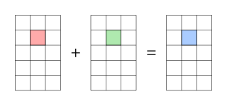
In mathematics, matrix addition is the operation of adding two matrices by adding the corresponding entries together.

In mathematics, particularly in linear algebra, matrix multiplication is a binary operation that produces a matrix from two matrices. For matrix multiplication, the number of columns in the first matrix must be equal to the number of rows in the second matrix. The resulting matrix, known as the matrix product, has the number of rows of the first and the number of columns of the second matrix. The product of matrices A and B is denoted as AB.

In mathematics, a square matrix is a matrix with the same number of rows and columns. An n-by-n matrix is known as a square matrix of order . Any two square matrices of the same order can be added and multiplied.
In linear algebra, a diagonal matrix is a matrix in which the entries outside the main diagonal are all zero; the term usually refers to square matrices. Elements of the main diagonal can either be zero or nonzero. An example of a 2×2 diagonal matrix is , while an example of a 3×3 diagonal matrix is. An identity matrix of any size, or any multiple of it is a diagonal matrix called a scalar matrix, for example, . In geometry, a diagonal matrix may be used as a scaling matrix, since matrix multiplication with it results in changing scale (size) and possibly also shape; only a scalar matrix results in uniform change in scale.
In linear algebra, an n-by-n square matrix A is called invertible if there exists an n-by-n square matrix B such that
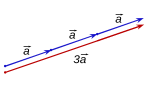
In mathematics, scalar multiplication is one of the basic operations defining a vector space in linear algebra. In common geometrical contexts, scalar multiplication of a real Euclidean vector by a positive real number multiplies the magnitude of the vector without changing its direction. Scalar multiplication is the multiplication of a vector by a scalar, and is to be distinguished from inner product of two vectors.
In linear algebra, a minor of a matrix A is the determinant of some smaller square matrix, cut down from A by removing one or more of its rows and columns. Minors obtained by removing just one row and one column from square matrices are required for calculating matrix cofactors, which in turn are useful for computing both the determinant and inverse of square matrices. The requirement that the square matrix be smaller than the original matrix is often omitted in the definition.
In linear algebra, a Vandermonde matrix, named after Alexandre-Théophile Vandermonde, is a matrix with the terms of a geometric progression in each row: an matrix
In mathematics, a triangular matrix is a special kind of square matrix. A square matrix is called lower triangular if all the entries above the main diagonal are zero. Similarly, a square matrix is called upper triangular if all the entries below the main diagonal are zero.

In mathematics, a block matrix or a partitioned matrix is a matrix that is interpreted as having been broken into sections called blocks or submatrices.
In linear algebra, a circulant matrix is a square matrix in which all rows are composed of the same elements and each row is rotated one element to the right relative to the preceding row. It is a particular kind of Toeplitz matrix.
In mathematics, the Smith normal form is a normal form that can be defined for any matrix with entries in a principal ideal domain (PID). The Smith normal form of a matrix is diagonal, and can be obtained from the original matrix by multiplying on the left and right by invertible square matrices. In particular, the integers are a PID, so one can always calculate the Smith normal form of an integer matrix. The Smith normal form is very useful for working with finitely generated modules over a PID, and in particular for deducing the structure of a quotient of a free module. It is named after the Irish mathematician Henry John Stephen Smith.
In numerical analysis and linear algebra, lower–upper (LU) decomposition or factorization factors a matrix as the product of a lower triangular matrix and an upper triangular matrix. The product sometimes includes a permutation matrix as well. LU decomposition can be viewed as the matrix form of Gaussian elimination. Computers usually solve square systems of linear equations using LU decomposition, and it is also a key step when inverting a matrix or computing the determinant of a matrix. The LU decomposition was introduced by the Polish astronomer Tadeusz Banachiewicz in 1938. To quote: "It appears that Gauss and Doolittle applied the method [of elimination] only to symmetric equations. More recent authors, for example, Aitken, Banachiewicz, Dwyer, and Crout … have emphasized the use of the method, or variations of it, in connection with non-symmetric problems … Banachiewicz … saw the point … that the basic problem is really one of matrix factorization, or “decomposition” as he called it." It is also sometimes referred to as LR decomposition.

In mathematics, a matrix is a rectangular array or table of numbers, symbols, or expressions, arranged in rows and columns, which is used to represent a mathematical object or a property of such an object.
In theoretical computer science, the computational complexity of matrix multiplication dictates how quickly the operation of matrix multiplication can be performed. Matrix multiplication algorithms are a central subroutine in theoretical and numerical algorithms for numerical linear algebra and optimization, so finding the fastest algorithm for matrix multiplication is of major practical relevance.
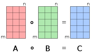
In mathematics, the Hadamard product is a binary operation that takes in two matrices of the same dimensions and returns a matrix of the multiplied corresponding elements. This operation can be thought as a "naive matrix multiplication" and is different from the matrix product. It is attributed to, and named after, either French mathematician Jacques Hadamard or German mathematician Issai Schur.


