
Supervised learning (SL) is the machine learning task of learning a function that maps an input to an output based on example input-output pairs. It infers a function from labeled training data consisting of a set of training examples. In supervised learning, each example is a pair consisting of an input object and a desired output value. A supervised learning algorithm analyzes the training data and produces an inferred function, which can be used for mapping new examples. An optimal scenario will allow for the algorithm to correctly determine the class labels for unseen instances. This requires the learning algorithm to generalize from the training data to unseen situations in a "reasonable" way. This statistical quality of an algorithm is measured through the so-called generalization error.

The principal components of a collection of points in a real coordinate space are a sequence of unit vectors, where the -th vector is the direction of a line that best fits the data while being orthogonal to the first vectors. Here, a best-fitting line is defined as one that minimizes the average squared distance from the points to the line. These directions constitute an orthonormal basis in which different individual dimensions of the data are linearly uncorrelated. Principal component analysis (PCA) is the process of computing the principal components and using them to perform a change of basis on the data, sometimes using only the first few principal components and ignoring the rest.
In machine learning, the perceptron is an algorithm for supervised learning of binary classifiers. A binary classifier is a function which can decide whether or not an input, represented by a vector of numbers, belongs to some specific class. It is a type of linear classifier, i.e. a classification algorithm that makes its predictions based on a linear predictor function combining a set of weights with the feature vector.

For statistics and control theory, Kalman filtering, also known as linear quadratic estimation (LQE), is an algorithm that uses a series of measurements observed over time, including statistical noise and other inaccuracies, and produces estimates of unknown variables that tend to be more accurate than those based on a single measurement alone, by estimating a joint probability distribution over the variables for each timeframe. The filter is named after Rudolf E. Kálmán, who was one of the primary developers of its theory.

High-dimensional data, meaning data that requires more than two or three dimensions to represent, can be difficult to interpret. One approach to simplification is to assume that the data of interest lies within lower-dimensional space. If the data of interest is of low enough dimension, the data can be visualised in the low-dimensional space.
Hebbian theory is a neuroscientific theory claiming that an increase in synaptic efficacy arises from a presynaptic cell's repeated and persistent stimulation of a postsynaptic cell. It is an attempt to explain synaptic plasticity, the adaptation of brain neurons during the learning process. It was introduced by Donald Hebb in his 1949 book The Organization of Behavior. The theory is also called Hebb's rule, Hebb's postulate, and cell assembly theory. Hebb states it as follows:
Let us assume that the persistence or repetition of a reverberatory activity tends to induce lasting cellular changes that add to its stability. ... When an axon of cell A is near enough to excite a cell B and repeatedly or persistently takes part in firing it, some growth process or metabolic change takes place in one or both cells such that A’s efficiency, as one of the cells firing B, is increased.
In signal processing, independent component analysis (ICA) is a computational method for separating a multivariate signal into additive subcomponents. This is done by assuming that the subcomponents are, potentially, non-Gaussian signals and that they are statistically independent from each other. ICA is a special case of blind source separation. A common example application is the "cocktail party problem" of listening in on one person's speech in a noisy room.
In Bayesian probability theory, if the posterior distribution p(θ | x) is in the same probability distribution family as the prior probability distribution p(θ), the prior and posterior are then called conjugate distributions, and the prior is called a conjugate prior for the likelihood function p(x | θ).
Tikhonov regularization, named for Andrey Tikhonov, is a method of regularization of ill-posed problems. Also known as ridge regression, it is particularly useful to mitigate the problem of multicollinearity in linear regression, which commonly occurs in models with large numbers of parameters. In general, the method provides improved efficiency in parameter estimation problems in exchange for a tolerable amount of bias.

Random forests or random decision forests are an ensemble learning method for classification, regression and other tasks that operates by constructing a multitude of decision trees at training time. For classification tasks, the output of the random forest is the class selected by most trees. For regression tasks, the mean or average prediction of the individual trees is returned. Random decision forests correct for decision trees' habit of overfitting to their training set. Random forests generally outperform decision trees, but their accuracy is lower than gradient boosted trees. However, data characteristics can affect their performance.
FastICA is an efficient and popular algorithm for independent component analysis invented by Aapo Hyvärinen at Helsinki University of Technology. Like most ICA algorithms, FastICA seeks an orthogonal rotation of prewhitened data, through a fixed-point iteration scheme, that maximizes a measure of non-Gaussianity of the rotated components. Non-gaussianity serves as a proxy for statistical independence, which is a very strong condition and requires infinite data to verify. FastICA can also be alternatively derived as an approximative Newton iteration.
In mathematics, a Relevance Vector Machine (RVM) is a machine learning technique that uses Bayesian inference to obtain parsimonious solutions for regression and probabilistic classification. The RVM has an identical functional form to the support vector machine, but provides probabilistic classification.
Oja's learning rule, or simply Oja's rule, named after Finnish computer scientist Erkki Oja, is a model of how neurons in the brain or in artificial neural networks change connection strength, or learn, over time. It is a modification of the standard Hebb's Rule that, through multiplicative normalization, solves all stability problems and generates an algorithm for principal components analysis. This is a computational form of an effect which is believed to happen in biological neurons.
The generalized Hebbian algorithm (GHA), also known in the literature as Sanger's rule, is a linear feedforward neural network model for unsupervised learning with applications primarily in principal components analysis. First defined in 1989, it is similar to Oja's rule in its formulation and stability, except it can be applied to networks with multiple outputs. The name originates because of the similarity between the algorithm and a hypothesis made by Donald Hebb about the way in which synaptic strengths in the brain are modified in response to experience, i.e., that changes are proportional to the correlation between the firing of pre- and post-synaptic neurons.
Non-linear least squares is the form of least squares analysis used to fit a set of m observations with a model that is non-linear in n unknown parameters (m ≥ n). It is used in some forms of nonlinear regression. The basis of the method is to approximate the model by a linear one and to refine the parameters by successive iterations. There are many similarities to linear least squares, but also some significant differences. In economic theory, the non-linear least squares method is applied in (i) the probit regression, (ii) threshold regression, (iii) smooth regression, (iv) logistic link regression, (v) Box-Cox transformed regressors.
In statistics and machine learning, ensemble methods use multiple learning algorithms to obtain better predictive performance than could be obtained from any of the constituent learning algorithms alone. Unlike a statistical ensemble in statistical mechanics, which is usually infinite, a machine learning ensemble consists of only a concrete finite set of alternative models, but typically allows for much more flexible structure to exist among those alternatives.
Backpropagation through time (BPTT) is a gradient-based technique for training certain types of recurrent neural networks. It can be used to train Elman networks. The algorithm was independently derived by numerous researchers.
In machine learning, the kernel perceptron is a variant of the popular perceptron learning algorithm that can learn kernel machines, i.e. non-linear classifiers that employ a kernel function to compute the similarity of unseen samples to training samples. The algorithm was invented in 1964, making it the first kernel classification learner.
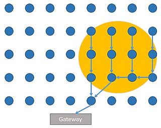
This article is about event detection for WSN.
Non-homogeneous Gaussian regression (NGR) is a type of statistical regression analysis used in the atmospheric sciences as a way to convert ensemble forecasts into probabilistic forecasts. Relative to simple linear regression, NGR uses the ensemble spread as an additional predictor, which is used to improve the prediction of uncertainty and allows the predicted uncertainty to vary from case to case. The prediction of uncertainty in NGR is derived from both past forecast errors statistics and the ensemble spread. NGR was originally developed for site-specific medium range temperature forecasting, but has since also been applied to site-specific medium-range wind forecasting and to seasonal forecasts, and has been adapted for precipitation forecasting. The introduction of NGR was the first demonstration that probabilistic forecasts that take account of the varying ensemble spread could achieve better skill scores than forecasts based on standard Model output statistics approaches applied to the ensemble mean.


