Econometrics is the application of statistical methods to economic data in order to give empirical content to economic relationships. More precisely, it is "the quantitative analysis of actual economic phenomena based on the concurrent development of theory and observation, related by appropriate methods of inference". An introductory economics textbook describes econometrics as allowing economists "to sift through mountains of data to extract simple relationships". Jan Tinbergen is one of the two founding fathers of econometrics. The other, Ragnar Frisch, also coined the term in the sense in which it is used today.
In statistics, the term linear model is used in different ways according to the context. The most common occurrence is in connection with regression models and the term is often taken as synonymous with linear regression model. However, the term is also used in time series analysis with a different meaning. In each case, the designation "linear" is used to identify a subclass of models for which substantial reduction in the complexity of the related statistical theory is possible.
In statistics, the Gauss–Markov theorem states that the ordinary least squares (OLS) estimator has the lowest sampling variance within the class of linear unbiased estimators, if the errors in the linear regression model are uncorrelated, have equal variances and expectation value of zero. The errors do not need to be normal, nor do they need to be independent and identically distributed. The requirement that the estimator be unbiased cannot be dropped, since biased estimators exist with lower variance. See, for example, the James–Stein estimator, ridge regression, or simply any degenerate estimator.

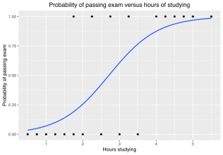
In statistics, the logistic model is a statistical model that models the probability of an event taking place by having the log-odds for the event be a linear combination of one or more independent variables. In regression analysis, logistic regression is estimating the parameters of a logistic model. Formally, in binary logistic regression there is a single binary dependent variable, coded by an indicator variable, where the two values are labeled "0" and "1", while the independent variables can each be a binary variable or a continuous variable. The corresponding probability of the value labeled "1" can vary between 0 and 1, hence the labeling; the function that converts log-odds to probability is the logistic function, hence the name. The unit of measurement for the log-odds scale is called a logit, from logistic unit, hence the alternative names. See § Background and § Definition for formal mathematics, and § Example for a worked example.

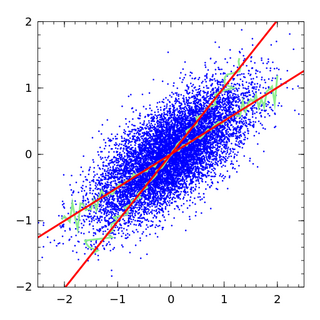
In statistics, Deming regression, named after W. Edwards Deming, is an errors-in-variables model which tries to find the line of best fit for a two-dimensional dataset. It differs from the simple linear regression in that it accounts for errors in observations on both the x- and the y- axis. It is a special case of total least squares, which allows for any number of predictors and a more complicated error structure.
In statistics and econometrics, and in particular in time series analysis, an autoregressive integrated moving average (ARIMA) model is a generalization of an autoregressive moving average (ARMA) model. Both of these models are fitted to time series data either to better understand the data or to predict future points in the series (forecasting). ARIMA models are applied in some cases where data show evidence of non-stationarity in the sense of mean, where an initial differencing step can be applied one or more times to eliminate the non-stationarity of the mean function. When the seasonality shows in a time series, the seasonal-differencing could be applied to eliminate the seasonal component. Since the ARMA model, according to the Wold's decomposition theorem, is theoretically sufficient to describe a regular wide-sense stationary time series, we are motivated to make stationary a non-stationary time series, e.g., by using differencing, before we can use the ARMA model. Note that if the time series contains a predictable sub-process, the predictable component is treated as a non-zero-mean but periodic component in the ARIMA framework so that it is eliminated by the seasonal differencing.
In statistics, ordinary least squares (OLS) is a type of linear least squares method for choosing the unknown parameters in a linear regression model by the principle of least squares: minimizing the sum of the squares of the differences between the observed dependent variable in the input dataset and the output of the (linear) function of the independent variable.
Cointegration is a statistical property of a collection (X1, X2, ..., Xk) of time series variables. First, all of the series must be integrated of order d. Next, if a linear combination of this collection is integrated of order less than d, then the collection is said to be co-integrated. Formally, if (X,Y,Z) are each integrated of order d, and there exist coefficients a,b,c such that aX + bY + cZ is integrated of order less than d, then X, Y, and Z are cointegrated. Cointegration has become an important property in contemporary time series analysis. Time series often have trends—either deterministic or stochastic. In an influential paper, Charles Nelson and Charles Plosser (1982) provided statistical evidence that many US macroeconomic time series have stochastic trends.
In econometrics, endogeneity broadly refers to situations in which an explanatory variable is correlated with the error term. The distinction between endogenous and exogenous variables originated in simultaneous equations models, where one separates variables whose values are determined by the model from variables which are predetermined; ignoring simultaneity in the estimation leads to biased estimates as it violates the exogeneity assumption of the Gauss–Markov theorem. The problem of endogeneity is often ignored by researchers conducting non-experimental research and doing so precludes making policy recommendations. Instrumental variable techniques are commonly used to address this problem.
Panel (data) analysis is a statistical method, widely used in social science, epidemiology, and econometrics to analyze two-dimensional panel data. The data are usually collected over time and over the same individuals and then a regression is run over these two dimensions. Multidimensional analysis is an econometric method in which data are collected over more than two dimensions.
In probability theory and statistics, a unit root is a feature of some stochastic processes that can cause problems in statistical inference involving time series models. A linear stochastic process has a unit root if 1 is a root of the process's characteristic equation. Such a process is non-stationary but does not always have a trend.
In statistics, the Dickey–Fuller test tests the null hypothesis that a unit root is present in an autoregressive time series model. The alternative hypothesis is different depending on which version of the test is used, but is usually stationarity or trend-stationarity. The test is named after the statisticians David Dickey and Wayne Fuller, who developed it in 1979.
The Chow test, proposed by econometrician Gregory Chow in 1960, is a test of whether the true coefficients in two linear regressions on different data sets are equal. In econometrics, it is most commonly used in time series analysis to test for the presence of a structural break at a period which can be assumed to be known a priori. In program evaluation, the Chow test is often used to determine whether the independent variables have different impacts on different subgroups of the population.
In statistics, the Breusch–Pagan test, developed in 1979 by Trevor Breusch and Adrian Pagan, is used to test for heteroskedasticity in a linear regression model. It was independently suggested with some extension by R. Dennis Cook and Sanford Weisberg in 1983. Derived from the Lagrange multiplier test principle, it tests whether the variance of the errors from a regression is dependent on the values of the independent variables. In that case, heteroskedasticity is present.
Cochrane–Orcutt estimation is a procedure in econometrics, which adjusts a linear model for serial correlation in the error term. Developed in the 1940s, it is named after statisticians Donald Cochrane and Guy Orcutt.
In statistics, the Ramsey Regression Equation Specification Error Test (RESET) test is a general specification test for the linear regression model. More specifically, it tests whether non-linear combinations of the fitted values help explain the response variable. The intuition behind the test is that if non-linear combinations of the explanatory variables have any power in explaining the response variable, the model is misspecified in the sense that the data generating process might be better approximated by a polynomial or another non-linear functional form.
In statistics, the Breusch–Godfrey test is used to assess the validity of some of the modelling assumptions inherent in applying regression-like models to observed data series. In particular, it tests for the presence of serial correlation that has not been included in a proposed model structure and which, if present, would mean that incorrect conclusions would be drawn from other tests or that sub-optimal estimates of model parameters would be obtained.

In statistics, errors-in-variables models or measurement error models are regression models that account for measurement errors in the independent variables. In contrast, standard regression models assume that those regressors have been measured exactly, or observed without error; as such, those models account only for errors in the dependent variables, or responses.
In statistics, the Johansen test, named after Søren Johansen, is a procedure for testing cointegration of several, say k, I(1) time series. This test permits more than one cointegrating relationship so is more generally applicable than the Engle–Granger test which is based on the Dickey–Fuller test for unit roots in the residuals from a single (estimated) cointegrating relationship.
In statistics, linear regression is a linear approach for modelling the relationship between a scalar response and one or more explanatory variables. The case of one explanatory variable is called simple linear regression; for more than one, the process is called multiple linear regression. This term is distinct from multivariate linear regression, where multiple correlated dependent variables are predicted, rather than a single scalar variable.


