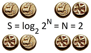
In information theory, the entropy of a random variable is the average level of "information", "surprise", or "uncertainty" inherent in the variable's possible outcomes. The concept of information entropy was introduced by Claude Shannon in his 1948 paper "A Mathematical Theory of Communication", and is sometimes called Shannon entropy in his honour. As an example, consider a biased coin with probability p of landing on heads and probability 1 − p of landing on tails. The maximum surprise is for p = 1/2, when there is no reason to expect one outcome over another, and in this case a coin flip has an entropy of one bit. The minimum surprise is when p = 0 or p = 1, when the event is known and the entropy is zero bits. Other values of p give different entropies between zero and one bits.
In statistics, the likelihood function measures the goodness of fit of a statistical model to a sample of data for given values of the unknown parameters. It is formed from the joint probability distribution of the sample, but viewed and used as a function of the parameters only, thus treating the random variables as fixed at the observed values.
In statistics, the likelihood-ratio test assesses the goodness of fit of two competing statistical models based on the ratio of their likelihoods, specifically one found by maximization over the entire parameter space and another found after imposing some constraint. If the constraint is supported by the observed data, the two likelihoods should not differ by more than sampling error. Thus the likelihood-ratio test tests whether this ratio is significantly different from one, or equivalently whether its natural logarithm is significantly different from zero.

The Pareto distribution, named after the Italian civil engineer, economist, and sociologist Vilfredo Pareto,, is a power-law probability distribution that is used in description of social, quality control, scientific, geophysical, actuarial, and many other types of observable phenomena. Originally applied to describing the distribution of wealth in a society, fitting the trend that a large portion of wealth is held by a small fraction of the population. The Pareto principle or "80-20 rule" stating that 80% of outcomes are due to 20% of causes was named in honour of Pareto, but the concepts are distinct, and only Pareto distributions with shape value of log45 ≈ 1.16 precisely reflect it. Empirical observation has shown that this 80-20 distribution fits a wide range of cases, including natural phenomena and human activities.

In probability theory and statistics, the chi-square distribution with k degrees of freedom is the distribution of a sum of the squares of k independent standard normal random variables. The chi-square distribution is a special case of the gamma distribution and is one of the most widely used probability distributions in inferential statistics, notably in hypothesis testing and in construction of confidence intervals. This distribution is sometimes called the central chi-square distribution, a special case of the more general noncentral chi-square distribution.
In statistics, maximum likelihood estimation (MLE) is a method of estimating the parameters of a probability distribution by maximizing a likelihood function, so that under the assumed statistical model the observed data is most probable. The point in the parameter space that maximizes the likelihood function is called the maximum likelihood estimate. The logic of maximum likelihood is both intuitive and flexible, and as such the method has become a dominant means of statistical inference.

In probability theory and statistics, the beta distribution is a family of continuous probability distributions defined on the interval [0, 1] parameterized by two positive shape parameters, denoted by α and β, that appear as exponents of the random variable and control the shape of the distribution. The generalization to multiple variables is called a Dirichlet distribution.
In statistics, the logistic model is used to model the probability of a certain class or event existing such as pass/fail, win/lose, alive/dead or healthy/sick. This can be extended to model several classes of events such as determining whether an image contains a cat, dog, lion, etc. Each object being detected in the image would be assigned a probability between 0 and 1, with a sum of one.
The power of a binary hypothesis test is denoted by "(1−β)" and is the probability of a "true positive". It is the probability that the test correctly rejects the null hypothesis when a specific alternative hypothesis is true. It is the probability of avoiding a "false negative", otherwise known as a type II error. The statistical power ranges from 0 to 1, and as statistical power increases, the size of "β" - the probability of making a type II error by wrongly failing to reject the null hypothesis - decreases.
The Akaike information criterion (AIC) is an estimator of prediction error and thereby relative quality of statistical models for a given set of data. Given a collection of models for the data, AIC estimates the quality of each model, relative to each of the other models. Thus, AIC provides a means for model selection.
In mathematical statistics, the Kullback–Leibler divergence,, is a measure of how one probability distribution is different from a second, reference probability distribution. Applications include characterizing the relative (Shannon) entropy in information systems, randomness in continuous time-series, and information gain when comparing statistical models of inference. In contrast to variation of information, it is a distribution-wise asymmetric measure and thus does not qualify as a statistical metric of spread – it also does not satisfy the triangle inequality. In the simple case, a relative entropy of 0 indicates that the two distributions in question have identical quantities of information. In simplified terms, it is a measure of surprise, with diverse applications such as applied statistics, fluid mechanics, neuroscience and bioinformatics.
Estimation theory is a branch of statistics that deals with estimating the values of parameters based on measured empirical data that has a random component. The parameters describe an underlying physical setting in such a way that their value affects the distribution of the measured data. An estimator attempts to approximate the unknown parameters using the measurements.
In statistics, ordinary least squares (OLS) is a type of linear least squares method for estimating the unknown parameters in a linear regression model. OLS chooses the parameters of a linear function of a set of explanatory variables by the principle of least squares: minimizing the sum of the squares of the differences between the observed dependent variable in the given dataset and those predicted by the linear function of the independent variable.
The goodness of fit of a statistical model describes how well it fits a set of observations. Measures of goodness of fit typically summarize the discrepancy between observed values and the values expected under the model in question. Such measures can be used in statistical hypothesis testing, e.g. to test for normality of residuals, to test whether two samples are drawn from identical distributions, or whether outcome frequencies follow a specified distribution. In the analysis of variance, one of the components into which the variance is partitioned may be a lack-of-fit sum of squares.
In statistics, the false discovery rate (FDR) is a method of conceptualizing the rate of type I errors in null hypothesis testing when conducting multiple comparisons. FDR-controlling procedures are designed to control the FDR, which is the expected proportion of "discoveries" that are false. Equivalently, the FDR is the expected ratio of the number of false positive classifications to the total number of positive classifications. The total number of rejections of the null include both the number of false positives (FP) and true positives (TP). Simply put, FDR = FP /. FDR-controlling procedures provide less stringent control of Type I errors compared to familywise error rate (FWER) controlling procedures, which control the probability of at least one Type I error. Thus, FDR-controlling procedures have greater power, at the cost of increased numbers of Type I errors.
In information theory, the error exponent of a channel code or source code over the block length of the code is the rate at which the error probability decays exponentially with the block length of the code. Formally, it is defined as the limiting ratio of the negative logarithm of the error probability to the block length of the code for large block lengths. For example, if the probability of error of a decoder drops as , where is the block length, the error exponent is . In this example, approaches for large . Many of the information-theoretic theorems are of asymptotic nature, for example, the channel coding theorem states that for any rate less than the channel capacity, the probability of the error of the channel code can be made to go to zero as the block length goes to infinity. In practical situations, there are limitations to the delay of the communication and the block length must be finite. Therefore, it is important to study how the probability of error drops as the block length go to infinity.
In probability theory, heavy-tailed distributions are probability distributions whose tails are not exponentially bounded: that is, they have heavier tails than the exponential distribution. In many applications it is the right tail of the distribution that is of interest, but a distribution may have a heavy left tail, or both tails may be heavy.
In statistics, when performing multiple comparisons, a false positive ratio is the probability of falsely rejecting the null hypothesis for a particular test. The false positive rate is calculated as the ratio between the number of negative events wrongly categorized as positive and the total number of actual negative events.
In probability theory, conditional probability is a measure of the probability of an event occurring, given that another event has already occurred. If the event of interest is A and the event B is known or assumed to have occurred, "the conditional probability of A given B", or "the probability of A under the condition B", is usually written as P(A|B), or sometimes PB(A) or P(A/B). For example, the probability that any given person has a cough on any given day may be only 5%. But if we know or assume that the person is sick, then they are much more likely to be coughing. For example, the conditional probability that someone unwell is coughing might be 75%, in which case we would have that P(Cough) = 5% and P(Cough|Sick) = 75%.
In statistics Wilks' theorem offers an asymptotic distribution of the log-likelihood ratio statistic, which can be used to produce confidence intervals for maximum-likelihood estimates or as a test statistic for performing the likelihood-ratio test.


