GLIMMER

GLIMMER

Developer(s)	Steven Salzberg & Arthur Delcher
Stable release	3.02 / 9 May 2006 (2006-05-09)
Available in	C++
Type	Bioinformatics tool
License	OSI Certified Open Source Software under the Artistic License
Website	ccb.jhu.edu/software/glimmer/index.shtml

In bioinformatics, GLIMMER (Gene Locator and Interpolated Markov ModelER) is used to find genes in prokaryotic DNA. ^[1] "It is effective at finding genes in bacteria, archea, viruses, typically finding 98-99% of all relatively long protein coding genes". ^[1] GLIMMER was the first system that used the interpolated Markov model ^[2] to identify coding regions. The GLIMMER software is open source and is maintained by Steven Salzberg, Art Delcher, and their colleagues at the Center for Computational Biology ^[3] at Johns Hopkins University. The original GLIMMER algorithms and software were designed by Art Delcher, Simon Kasif and Steven Salzberg and applied to bacterial genome annotation in collaboration with Owen White.

Versions

GLIMMER 1.0

First Version of GLIMMER "i.e., GLIMMER 1.0" was released in 1998 and it was published in the paper Microbial gene identification using interpolated Markov model. ^[1] Markov models were used to identify microbial genes in GLIMMER 1.0. GLIMMER considers the local composition sequence dependencies which makes GLIMMER more flexible and more powerful when compared to fixed-order Markov model.

There was a comparison made between interpolated Markov model used by GLIMMER and fifth order Markov model in the paper Microbial gene identification using interpolated Markov models. ^[1] "GLIMMER algorithm found 1680 genes out of 1717 annotated genes in Haemophilus influenzae where fifth order Markov model found 1574 genes. GLIMMER found 209 additional genes which were not included in 1717 annotated genes where fifth order Markov model found 104 genes."' ^[1]

GLIMMER 2.0

Second Version of GLIMMER i.e., GLIMMER 2.0 was released in 1999 and it was published in the paper Improved microbial identification with GLIMMER. ^[4] This paper ^[4] provides significant technical improvements such as using interpolated context model instead of interpolated Markov model and resolving overlapping genes which improves the accuracy of GLIMMER.

Interpolated context models are used instead of interpolated Markov model which gives the flexibility to select any base. In interpolated Markov model probability distribution of a base is determined from the immediate preceding bases. If the immediate preceding base is irrelevant amino acid translation, interpolated Markov model still considers the preceding base to determine the probability of given base where as interpolated context model which was used in GLIMMER 2.0 can ignore irrelevant bases. False positive predictions were increased in GLIMMER 2.0 to reduce the number of false negative predictions. Overlapped genes are also resolved in GLIMMER 2.0.

Various comparisons between GLIMMER 1.0 and GLIMMER 2.0 were made in the paper Improved microbial identification with GLIMMER ^[4] which shows improvement in the later version. "Sensitivity of GLIMMER 1.0 ranges from 98.4 to 99.7% with an average of 99.1% where as GLIMMER 2.0 has a sensitivity range from 98.6 to 99.8% with an average of 99.3%. GLIMMER 2.0 is very effective in finding genes of high density. The parasite Trypanosoma brucei, responsible for causing African sleeping sickness is being identified by GLIMMER 2.0" ^[4]

GLIMMER 3.0

Third version of GLIMMER, "GLIMMER 3.0" was released in 2007 and it was published in the paper Identifying bacterial genes and endosymbiont DNA with Glimmer. ^[5] This paper describes several major changes made to the GLIMMER system including improved methods to identify coding regions and start codon. Scoring of ORF in GLIMMER 3.0 is done in reverse order i.e., starting from stop codon and moves back towards the start codon. Reverse scanning helps in identifying the coding portion of the gene more accurately which is contained in the context window of IMM. GLIMMER 3.0 also improves the generated training set data by comparing the long-ORF with universal amino acid distribution of widely disparate bacterial genomes."GLIMMER 3.0 has an average long-ORF output of 57% for various organisms where as GLIMMER 2.0 has an average long-ORF output of 39%." ^[5]

GLIMMER 3.0 reduces the rate of false positive predictions which were increased in GLIMMER 2.0 to reduce the number of false negative predictions. "GLIMMER 3.0 has a start-site prediction accuracy of 99.5% for 3'5' matches where as GLIMMER 2.0 has 99.1% for 3'5' matches. GLIMMER 3.0 uses a new algorithm for scanning coding regions, a new start site detection module, and architecture which integrates all gene predictions across an entire genome." ^[5]

Minimum description length

Theoretical and Biological Foundation

The GLIMMER project helped introduce and popularize the use of variable length models in Computational Biology and Bioinformatics that subsequently have been applied to numerous problems such as protein classification and others. Variable length modeling was originally pioneered by information theorists and subsequently ingeniously applied and popularized in data compression (e.g. Ziv-Lempel compression). Prediction and compression are intimately linked using Minimum Description Length Principles. The basic idea is to create a dictionary of frequent words (motifs in biological sequences). The intuition is that the frequently occurring motifs are likely to be most predictive and informative. In GLIMMER the interpolated model is a mixture model of the probabilities of these relatively common motifs. Similarly to the development of HMMs in Computational Biology, the authors of GLIMMER were conceptually influenced by the previous application of another variant of interpolated Markov models to speech recognition by researchers such as Fred Jelinek (IBM) and Eric Ristad (Princeton). The learning algorithm in GLIMMER is different from these earlier approaches.

Access

GLIMMER can be downloaded from The Glimmer home page (requires a C++ compiler). Alternatively, an online version is hosted by NCBI .

How it works

1. GLIMMER primarily searches for long-ORFS. An open reading frame might overlap with any other open reading frame which will be resolved using the technique described in the sub section. Using these long-ORFS and following certain amino acid distribution GLIMMER generates training set data.
2. Using these training data, GLIMMER trains all the six Markov models of coding DNA from zero to eight order and also train the model for noncoding DNA
3. GLIMMER tries to calculate the probabilities from the data. Based on the number of observations, GLIMMER determines whether to use fixed order Markov model or interpolated Markov model.
   1. If the number of observations are greater than 400, GLIMMER uses fixed order Markov model to obtain there probabilities.
   2. If the number of observations are less than 400, GLIMMER uses interpolated Markov model which is briefly explained in the next sub section.
4. GLIMMER obtains score for every long-ORF generated using all the six coding DNA models and also using non-coding DNA model.
5. If the score obtained in the previous step is greater than a certain threshold then GLIMMER predicts it to be a gene.

The steps explained above describes the basic functionality of GLIMMER. There are various improvements made to GLIMMER and some of them are described in the following sub-sections.

The GLIMMER system

GLIMMER system consists of two programs. First program called build-imm, which takes an input set of sequences and outputs the interpolated Markov model as follows.

The probability for each base i.e., A,C,G,T for all k-mers for 0 ≤ k ≤ 8 is computed. Then, for each k-mer, GLIMMER computes weight. New sequence probability is computed as follows.

${\displaystyle \operatorname {P(S|M)=\sum _{x=1}^{n}{IMM_{8}(S_{x})}} }$

where n is the length of the sequence ${\displaystyle S_{x}}$ is the oligomer at position x. ${\displaystyle IMM_{8}(S_{x})}$, the ${\displaystyle 8^{th}}$-order interpolated Markov model score is computed as

${\displaystyle \operatorname {IMM_{k}(S_{x})=Y_{k}(S_{x-1})\cdot P_{k}(S_{x})+[1-{Y_{k}(S_{x-1})]\cdot IMM_{k-1}(S_{x})}} }$

"where ${\displaystyle Y_{k}(S_{x-1})}$ is the weight of the k-mer at position x-1 in the sequence S and ${\displaystyle P_{k}(S_{x})}$ is the estimate obtained from the training data of the probability of the base located at position x in the ${\displaystyle k^{th}}$-order model." ^[1]

The probability of base ${\displaystyle S_{x}}$ given the i previous bases is computed as follows.

${\displaystyle \operatorname {P_{i}(S_{x})=P(s_{x}|S_{x,j})={\frac {f(S_{x,j})}{\sum _{b\in {[acgt]}}\operatorname {f(S_{x,i},b)} }}} }$

"The value of ${\displaystyle Y_{i}(S_{x})}$ associated with ${\displaystyle P_{i}(S_{x})}$ can be regarded as a measure of confidence in the accuracy of this value as an estimate of the true probability. GLIMMER uses two criteria to determine ${\displaystyle Y_{i}(S_{x})}$. The first of these is simple frequency occurrence in which the number of occurrences of context string ${\displaystyle S_{x,i}}$ in the training data exceeds a specific threshold value, then ${\displaystyle Y_{i}(S_{x})}$ is set to 1.0. The current default value for threshold is 400, which gives 95% confidence. When there are insufficient sample occurrences of a context string, build-imm employ additional criteria to determine ${\displaystyle Y}$ value. For a given context string ${\displaystyle S_{x,i}}$ of length i, build-imm compare the observed frequencies of the following base ${\displaystyle f(S_{x,i},a)}$, ${\displaystyle f(S_{x,i},c)}$, ${\displaystyle f(S_{x,i},g)}$, ${\displaystyle f(S_{x,i},t)}$ with the previously calculated interpolated Markov model probabilities using the next shorter context, ${\displaystyle IMM_{i-1}(S_{x,{i-1}},a)}$, ${\displaystyle IMM_{i-1}(S_{x,{i-1}},c)}$, ${\displaystyle IMM_{i-1}(S_{x,{i-1}},g)}$, ${\displaystyle IMM_{i-1}(S_{x,{i-1}},t)}$. Using a ${\displaystyle X^{2}}$ test, build-imm determine how likely it is that the four observed frequencies are consistent with the IMM values from the next shorter context." ^[1]

The second program called glimmer, then uses this IMM to identify putative gene in an entire genome. GLIMMER identifies all the open reading frame which score higher than threshold and check for overlapping genes. Resolving overlapping genes is explained in the next sub-section.

Equations and explanation of the terms used above are taken from the paper 'Microbial gene identification using interpolated Markov models ^[1]

Resolving overlapping genes

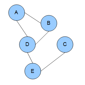
In GLIMMER 1.0, when two genes A and B overlap, the overlap region is scored. If A is longer than B, and if A scores higher on the overlap region, and if moving B's start site will not resolve the overlap, then B is rejected.

GLIMMER 2.0 provided a better solution to resolve the overlap. In GLIMMER 2.0, when two potential genes A and B overlap, the overlap region is scored. Suppose gene A scores higher, four different orientations are considered.

Case 1

In the above case, moving of start sites does not remove the overlap. If A is significantly longer than B, then B is rejected or else both A and B are called genes, with a doubtful overlap.

Case 2

In the above case, moving of B can resolve the overlap, A and B can be called non overlapped genes but if B is significantly shorter than A, then B is rejected.

Case 3

In the above case, moving of A can resolve the overlap. A is only moved if overlap is a small fraction of A or else B is rejected.

Case 4

In the above case, both A and B can be moved. We first move the start of B until the overlap region scores higher for B. Then we move the start of A until it scores higher. Then B again, and so on, until either the overlap is eliminated or no further moves can be made.

The above example has been taken from the paper 'Identifying bacterial genes and endosymbiont DNA with Glimmer' ^[5]

Ribosome binding sites

Ribosome binding site(RBS) signal can be used to find true start site position. GLIMMER results are passed as an input for RBSfinder program to predict ribosome binding sites. GLIMMER 3.0 integrates RBSfinder program into gene predicting function itself.

ELPH software( which was determined as highly effective at identifying RBS in the paper ^[5] ) is used for identifying RBS and is available at this website Archived 2013-11-27 at the Wayback Machine . Gibbs sampling algorithm is used to identify shared motif in any set of sequences. This shared motif sequences and their length is given as input to ELPH. ELPH then computes the position weight matrix(PWM) which will be used by GLIMMER 3 to score any potential RBS found by RBSfinder. The above process is done when we have a substantial amount of training genes. If there are inadequate number of training genes, GLIMMER 3 can bootstrap itself to generate a set of gene predictions which can be used as input to ELPH. ELPH now computes PWM and this PWM can be again used on the same set of genes to get more accurate results for start-sites. This process can be repeated for many iterations to obtain more consistent PWM and gene prediction results.

Performance

Glimmer supports genome annotation efforts on a wide range of bacterial, archaeal, and viral species. In a large-scale reannotation effort at the DNA Data Bank of Japan (DDBJ, which mirrors Genbank). Kosuge et al. (2006) ^[6] examined the gene finding methods used for 183 genomes. They reported that of these projects, Glimmer was the gene finder for 49%, followed by GeneMark with 12%, with other algorithms used in 3% or fewer of the projects. (They also reported that 33% of genomes used "other" programs, which in many cases meant that they could not identify the method. Excluding those cases, Glimmer was used for 73% of the genomes for which the methods could be unambiguously identified.) Glimmer was used by the DDBJ to re-annotate all bacterial genomes in the International Nucleotide Sequence Databases. ^[7] It is also being used by this group to annotate viruses. ^[8] Glimmer is part of the bacterial annotation pipeline at the National Center for Biotechnology Information (NCBI), ^[9] which also maintains a web server for Glimmer, ^[10] as do sites in Germany, ^[11] Canada. ^[12]

According to Google Scholar, as of early 2011 the original Glimmer article (Salzberg et al., 1998) ^[1] has been cited 581 times, and the Glimmer 2.0 article (Delcher et al., 1999) ^[4] has been cited 950 times.

References

1. Salzberg, S. L.; Delcher, A. L.; Kasif, S.; White, O. (1998). "Microbial gene identification using interpolated Markov models". Nucleic Acids Research. 26 (2): 544–548. doi:10.1093/nar/26.2.544. PMC   147303 . PMID   9421513.
2. Salzberg, S. L.; Pertea, M.; Delcher, A. L.; Gardner, M. J.; Tettelin, H. (1999). "Interpolated Markov Models for Eukaryotic Gene Finding". Genomics. 59 (1): 24–31. CiteSeerX   10.1.1.126.431 . doi:10.1006/geno.1999.5854. PMID   10395796.
3. "Center for Computational Biology". Johns Hopkins University. Retrieved 23 March 2013.
4. Delcher, A.; Harmon, D.; Kasif, S.; White, O.; Salzberg, S. (1999). "Improved microbial gene identification with GLIMMER". Nucleic Acids Research. 27 (23): 4636–4641. doi:10.1093/nar/27.23.4636. PMC   148753 . PMID   10556321.
5. Delcher, A. L.; Bratke, K. A.; Powers, E. C.; Salzberg, S. L. (2007). "Identifying bacterial genes and endosymbiont DNA with Glimmer". Bioinformatics. 23 (6): 673–679. doi:10.1093/bioinformatics/btm009. PMC   2387122 . PMID   17237039.
6. Kosuge, T.; Abe, T.; Okido, T.; Tanaka, N.; Hirahata, M.; Maruyama, Y.; Mashima, J.; Tomiki, A.; Kurokawa, M.; Himeno, R.; Fukuchi, S.; Miyazaki, S.; Gojobori, T.; Tateno, Y.; Sugawara, H. (2006). "Exploration and Grading of Possible Genes from 183 Bacterial Strains by a Common Protocol to Identification of New Genes: Gene Trek in Prokaryote Space (GTPS)". DNA Research. 13 (6): 245–254. doi: 10.1093/dnares/dsl014 . PMID   17166861.
7. Sugawara, H.; Abe, T.; Gojobori, T.; Tateno, Y. (2007). "DDBJ working on evaluation and classification of bacterial genes in INSDC". Nucleic Acids Research. 35 (Database issue): D13–D15. doi:10.1093/nar/gkl908. PMC   1669713 . PMID   17108353.
8. Hirahata, M.; Abe, T.; Tanaka, N.; Kuwana, Y.; Shigemoto, Y.; Miyazaki, S.; Suzuki, Y.; Sugawara, H. (2007). "Genome Information Broker for Viruses (GIB-V): Database for comparative analysis of virus genomes". Nucleic Acids Research. 35 (Database issue): D339–D342. doi:10.1093/nar/gkl1004. PMC   1781101 . PMID   17158166.
9. "NCBI Prokaryotic Genomes Automatic Annotation Pipeline (PGAAP)". Center for Bioinformatics and Computational Biology. Retrieved 23 March 2012.
10. "Microbial Genome Annotation Tools". Center for Bioinformatics and Computational Biology. Retrieved 23 March 2012.
11. "TiCo". Institut für Mikrobiologie und Genetik, Universität Göttingen. 2005-02-11. Archived from the original on 2022-03-31. Retrieved 23 March 2012.
12. "BASys Bacterial Annotation System". Archived from the original on 24 July 2012. Retrieved 23 March 2012.

External links

• The Glimmer home page at CCB, Johns Hopkins University, from which the software can be downloaded.