Geodesics on an ellipsoid

A geodesic on an oblate ellipsoid

The study of geodesics on an ellipsoid arose in connection with geodesy specifically with the solution of triangulation networks. The figure of the Earth is well approximated by an oblate ellipsoid , a slightly flattened sphere. A geodesic is the shortest path between two points on a curved surface, analogous to a straight line on a plane surface. The solution of a triangulation network on an ellipsoid is therefore a set of exercises in spheroidal trigonometry ( Euler 1755 ).

If the Earth is treated as a sphere, the geodesics are great circles (all of which are closed) and the problems reduce to ones in spherical trigonometry. However, Newton (1687) showed that the effect of the rotation of the Earth results in its resembling a slightly oblate ellipsoid: in this case, the equator and the meridians are the only simple closed geodesics. Furthermore, the shortest path between two points on the equator does not necessarily run along the equator. Finally, if the ellipsoid is further perturbed to become a triaxial ellipsoid (with three distinct semi-axes), only three geodesics are closed.

Geodesics on an ellipsoid of revolution

There are several ways of defining geodesics ( Hilbert & Cohn-Vossen 1952 , pp. 220–221 ). A simple definition is as the shortest path between two points on a surface. However, it is frequently more useful to define them as paths with zero geodesic curvature—i.e., the analogue of straight lines on a curved surface. This definition encompasses geodesics traveling so far across the ellipsoid's surface that they start to return toward the starting point, so that other routes are more direct, and includes paths that intersect or re-trace themselves. Short enough segments of a geodesics are still the shortest route between their endpoints, but geodesics are not necessarily globally minimal (i.e. shortest among all possible paths). Every globally-shortest path is a geodesic, but not vice versa.

By the end of the 18th century, an ellipsoid of revolution (the term spheroid is also used) was a well-accepted approximation to the figure of the Earth. The adjustment of triangulation networks entailed reducing all the measurements to a reference ellipsoid and solving the resulting two-dimensional problem as an exercise in spheroidal trigonometry ( Bomford 1952 , Chap. 3)( Leick et al. 2015 , §4.5).

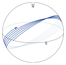
Fig. 1. A geodesic AB on an ellipsoid of revolution. N is the north pole and EFH lie on the equator.

It is possible to reduce the various geodesic problems into one of two types. Consider two points: A at latitude φ₁ and longitude λ₁ and B at latitude φ₂ and longitude λ₂ (see Fig. 1). The connecting geodesic (from A to B) is AB, of length s₁₂, which has azimuths α₁ and α₂ at the two endpoints. ^[1] The two geodesic problems usually considered are:

1. the direct geodesic problem or first geodesic problem, given A, α₁, and s₁₂, determine B and α₂;
2. the inverse geodesic problem or second geodesic problem, given A and B, determine s₁₂, α₁, and α₂.

As can be seen from Fig. 1, these problems involve solving the triangle NAB given one angle, α₁ for the direct problem and λ₁₂ = λ₂−λ₁ for the inverse problem, and its two adjacent sides. For a sphere the solutions to these problems are simple exercises in spherical trigonometry, whose solution is given by formulas for solving a spherical triangle. (See the article on great-circle navigation.)

For an ellipsoid of revolution, the characteristic constant defining the geodesic was found by Clairaut (1735). A systematic solution for the paths of geodesics was given by Legendre (1806) and Oriani (1806) (and subsequent papers in 1808 and 1810). The full solution for the direct problem (complete with computational tables and a worked out example) is given by Bessel (1825).

During the 18th century geodesics were typically referred to as "shortest lines". The term "geodesic line" (actually, a curve) was coined by Laplace (1799b):

Nous désignerons cette ligne sous le nom de ligne géodésique [We will call this line the geodesic line].

This terminology was introduced into English either as "geodesic line" or as "geodetic line", for example ( Hutton 1811 , p. 115 ),

A line traced in the manner we have now been describing, or deduced from trigonometrical measures, by the means we have indicated, is called a geodetic or geodesic line: it has the property of being the shortest which can be drawn between its two extremities on the surface of the Earth; and it is therefore the proper itinerary measure of the distance between those two points.

In its adoption by other fields geodesic line, frequently shortened to geodesic, was preferred.

This section treats the problem on an ellipsoid of revolution (both oblate and prolate). The problem on a triaxial ellipsoid is covered in the next section.

Equations for a geodesic

Fig. 2. Differential element of a meridian ellipse.

Fig. 3. Differential element of a geodesic on an ellipsoid.

Here the equations for a geodesic are developed; the derivation closely follows that of Bessel (1825). Jordan & Eggert (1941), Bagratuni (1962 , §15), Gan'shin (1967 , Chap. 5), Krakiwsky & Thomson (1974 , §4), Rapp (1993 , §1.2), Jekeli (2012), and Borre & Strang (2012) also provide derivations of these equations.

Consider an ellipsoid of revolution with equatorial radius a and polar semi-axis b. Define the flattening f, the eccentricity e, and the second eccentricity e′:

${\displaystyle f={\frac {a-b}{a}},\quad e={\frac {\sqrt {a^{2}-b^{2}}}{a}}={\sqrt {f(2-f)}},\quad e'={\frac {\sqrt {a^{2}-b^{2}}}{b}}={\frac {e}{1-f}}.}$

(In most applications in geodesy, the ellipsoid is taken to be oblate, a>b; however, the theory applies without change to prolate ellipsoids, a<b, in which case f, e², and e′² are negative.)

Let an elementary segment of a path on the ellipsoid have length ds. From Figs. 2 and 3, we see that if its azimuth is α, then ds is related to dφ and dλ by

${\displaystyle \cos \alpha \,ds=\rho \,d\varphi =-{\frac {dR}{\sin \varphi }},\quad \sin \alpha \,ds=R\,d\lambda ,}$(1)

where ρ is the meridional radius of curvature, R = ν cosφ is the radius of the circle of latitude φ, and ν is the normal radius of curvature. The elementary segment is therefore given by

${\displaystyle ds^{2}=\rho ^{2}\,d\varphi ^{2}+R^{2}\,d\lambda ^{2}}$

or

${\displaystyle {\begin{aligned}ds&={\sqrt {\rho ^{2}\varphi '^{2}+R^{2}}}\,d\lambda \\&\equiv L(\varphi ,\varphi ')\,d\lambda ,\end{aligned}}}$

where φ′ = dφ/dλ and the Lagrangian function L depends on φ through ρ(φ) and R(φ). The length of an arbitrary path between (φ₁, λ₁) and (φ₂, λ₂) is given by

${\displaystyle s_{12}=\int _{\lambda _{1}}^{\lambda _{2}}L(\varphi ,\varphi ')\,d\lambda ,}$

where φ is a function of λ satisfying φ(λ₁) = φ₁ and φ(λ₂) = φ₂. The shortest path or geodesic entails finding that function φ(λ) which minimizes s₁₂. This is an exercise in the calculus of variations and the minimizing condition is given by the Beltrami identity,

${\displaystyle L-\varphi '{\frac {\partial L}{\partial \varphi '}}={\text{const.}}}$

Substituting for L and using Eqs. (1) gives

${\displaystyle R\sin \alpha ={\text{const.}}}$

Clairaut (1735) found this relation, using a geometrical construction; a similar derivation is presented by Lyusternik (1964 , §10). ^[2] Differentiating this relation gives

${\displaystyle d\alpha =\sin \varphi \,d\lambda .}$

This, together with Eqs. (1) , leads to a system of ordinary differential equations for a geodesic

${\displaystyle {\frac {d\varphi }{ds}}={\frac {\cos \alpha }{\rho }};\quad {\frac {d\lambda }{ds}}={\frac {\sin \alpha }{\nu \cos \varphi }};\quad {\frac {d\alpha }{ds}}={\frac {\tan \varphi \sin \alpha }{\nu }}.}$

We can express R in terms of the parametric latitude, β, using

${\displaystyle R=a\cos \beta ,}$

and Clairaut's relation then becomes

${\displaystyle \sin \alpha _{1}\cos \beta _{1}=\sin \alpha _{2}\cos \beta _{2}.}$

Fig. 4. Geodesic problem mapped to the auxiliary sphere.

Fig. 5. The elementary geodesic problem on the auxiliary sphere.

This is the sine rule of spherical trigonometry relating two sides of the triangle NAB (see Fig. 4), NA = 1⁄2π−β₁, and NB = 1⁄2π−β₂ and their opposite angles B = π−α₂ and A = α₁.

In order to find the relation for the third side AB = σ₁₂, the spherical arc length, and included angle N = ω₁₂, the spherical longitude, it is useful to consider the triangle NEP representing a geodesic starting at the equator; see Fig. 5. In this figure, the variables referred to the auxiliary sphere are shown with the corresponding quantities for the ellipsoid shown in parentheses. Quantities without subscripts refer to the arbitrary point P; E, the point at which the geodesic crosses the equator in the northward direction, is used as the origin for σ, s and ω.

Fig. 6. Differential element of a geodesic on a sphere.

If the side EP is extended by moving P infinitesimally (see Fig. 6), we obtain

${\displaystyle \cos \alpha \,d\sigma =d\beta ,\quad \sin \alpha \,d\sigma =\cos \beta \,d\omega .}$(2)

Combining Eqs. (1) and (2) gives differential equations for s and λ

${\displaystyle {\frac {1}{a}}{\frac {ds}{d\sigma }}={\frac {d\lambda }{d\omega }}={\frac {\sin \beta }{\sin \varphi }}.}$

The relation between β and φ is

${\displaystyle \tan \beta ={\sqrt {1-e^{2}}}\tan \varphi =(1-f)\tan \varphi ,}$

which gives

${\displaystyle {\frac {\sin \beta }{\sin \varphi }}={\sqrt {1-e^{2}\cos ^{2}\beta }},}$

so that the differential equations for the geodesic become

${\displaystyle {\frac {1}{a}}{\frac {ds}{d\sigma }}={\frac {d\lambda }{d\omega }}={\sqrt {1-e^{2}\cos ^{2}\beta }}.}$

The last step is to use σ as the independent parameter in both of these differential equations and thereby to express s and λ as integrals. Applying the sine rule to the vertices E and G in the spherical triangle EGP in Fig. 5 gives

${\displaystyle \sin \beta =\sin \beta (\sigma$ ;\alpha _{0})=\cos \alpha _{0}\sin \sigma ,}

where α₀ is the azimuth at E. Substituting this into the equation for ds/d σ and integrating the result gives

${\displaystyle {\frac {s}{b}}=\int _{0}^{\sigma }{\sqrt {1+k^{2}\sin ^{2}\sigma '}}\,d\sigma ',}$(3)

where

${\displaystyle k=e'\cos \alpha _{0},}$

and the limits on the integral are chosen so that s(σ = 0) = 0. Legendre (1811 , p. 180 ) pointed out that the equation for s is the same as the equation for the arc on an ellipse with semi-axes b√1 + e′² cos²α₀ and b. In order to express the equation for λ in terms of σ, we write

${\displaystyle d\omega ={\frac {\sin \alpha _{0}}{\cos ^{2}\beta }}\,d\sigma ,}$

which follows from Eq. 2 and Clairaut's relation. This yields

${\displaystyle \lambda -\lambda _{0}=\omega -f\sin \alpha _{0}\int _{0}^{\sigma }{\frac {2-f}{1+(1-f){\sqrt {1+k^{2}\sin ^{2}\sigma '}}}}\,d\sigma ',}$(4)

and the limits on the integrals are chosen so that λ = λ₀ at the equator crossing, σ = 0.

This completes the solution of the path of a geodesic using the auxiliary sphere. By this device a great circle can be mapped exactly to a geodesic on an ellipsoid of revolution.

There are also several ways of approximating geodesics on a terrestrial ellipsoid (with small flattening) ( Rapp 1991 , §6); some of these are described in the article on geographical distance. However, these are typically comparable in complexity to the method for the exact solution ( Jekeli 2012 , §2.1.4).

Behavior of geodesics

Fig. 7. Meridians and the equator are the only closed geodesics. (For the very flattened ellipsoids, there are other closed geodesics; see Figs. 11 and 12).

Geodesic on an oblate ellipsoid (f = 1⁄50) with α₀ = 45°.

Fig. 8. Following the geodesic on the ellipsoid for about 5 circuits.

Fig. 9. The same geodesic after about 70 circuits.

Fig. 10. Geodesic on a prolate ellipsoid (f = −1⁄50) with α₀ = 45°. Compare with Fig. 8.

Fig. 7 shows the simple closed geodesics which consist of the meridians (green) and the equator (red). (Here the qualification "simple" means that the geodesic closes on itself without an intervening self-intersection.) This follows from the equations for the geodesics given in the previous section.

All other geodesics are typified by Figs. 8 and 9 which show a geodesic starting on the equator with α₀ = 45°. The geodesic oscillates about the equator. The equatorial crossings are called nodes and the points of maximum or minimum latitude are called vertices; the parametric latitudes of the vertices are given by β = ±(1⁄2π− |α₀|). The geodesic completes one full oscillation in latitude before the longitude has increased by 360°. Thus, on each successive northward crossing of the equator (see Fig. 8), λ falls short of a full circuit of the equator by approximately 2πf sinα₀ (for a prolate ellipsoid, this quantity is negative and λ completes more that a full circuit; see Fig. 10). For nearly all values of α₀, the geodesic will fill that portion of the ellipsoid between the two vertex latitudes (see Fig. 9).

Two additional closed geodesics for the oblate ellipsoid, b⁄a = 2⁄7.

Fig. 11. Side view.

Fig. 12. Top view.

If the ellipsoid is sufficiently oblate, i.e., b⁄a<1⁄2, another class of simple closed geodesics is possible ( Klingenberg 1982 , §3.5.19). Two such geodesics are illustrated in Figs. 11 and 12. Here b⁄a = 2⁄7 and the equatorial azimuth, α₀, for the green (resp. blue) geodesic is chosen to be 53.175° (resp. 75.192°), so that the geodesic completes 2 (resp. 3) complete oscillations about the equator on one circuit of the ellipsoid.

Fig. 13. Geodesics (blue) from a single point for f = 1⁄10, φ₁ = −30°; geodesic circles are shown in green and the cut locus in red.

Fig. 13 shows geodesics (in blue) emanating A with α₁ a multiple of 15° up to the point at which they cease to be shortest paths. (The flattening has been increased to 1⁄10 in order to accentuate the ellipsoidal effects.) Also shown (in green) are curves of constant s₁₂, which are the geodesic circles centered A. Gauss (1828) showed that, on any surface, geodesics and geodesic circle intersect at right angles. The red line is the cut locus, the locus of points which have multiple (two in this case) shortest geodesics from A. On a sphere, the cut locus is a point. On an oblate ellipsoid (shown here), it is a segment of the circle of latitude centered on the point antipodal to A, φ = −φ₁. The longitudinal extent of cut locus is approximately λ₁₂∈ [π−fπ cosφ₁, π + fπ cosφ₁]. If A lies on the equator, φ₁ = 0, this relation is exact and as a consequence the equator is only a shortest geodesic if |λ₁₂| ≤ (1 −f)π. For a prolate ellipsoid, the cut locus is a segment of the anti-meridian centered on the point antipodal to A, λ₁₂ = π, and this means that meridional geodesics stop being shortest paths before the antipodal point is reached.

Differential properties of geodesics

Various problems involving geodesics require knowing their behavior when they are perturbed. This is useful in trigonometric adjustments ( Ehlert 1993 ), determining the physical properties of signals which follow geodesics, etc. Consider a reference geodesic, parameterized by s, and a second geodesic a small distance t(s) away from it. Gauss (1828) showed that t(s) obeys the Gauss-Jacobi equation

${\displaystyle {\frac {d^{2}t(s)}{ds^{2}}}+K(s)t(s)=0,}$

Fig. 14. Definition of reduced length and geodesic scale.

where K(s) is the Gaussian curvature at s. As a second order, linear, homogeneous differential equation, its solution may be expressed as the sum of two independent solutions

${\displaystyle t(s_{2})=Cm(s_{1},s_{2})+DM(s_{1},s_{2})}$

where

${\displaystyle {\begin{aligned}m(s_{1},s_{1})&=0,\quad \left.{\frac {dm(s_{1},s_{2})}{ds_{2}}}\right|_{s_{2}=s_{1}}=1,\\M(s_{1},s_{1})&=1,\quad \left.{\frac {dM(s_{1},s_{2})}{ds_{2}}}\right|_{s_{2}=s_{1}}=0.\end{aligned}}}$

The quantity m(s₁, s₂) = m₁₂ is the so-called reduced length, and M(s₁, s₂) = M₁₂ is the geodesic scale. ^[3] Their basic definitions are illustrated in Fig. 14.

The Gaussian curvature for an ellipsoid of revolution is

${\displaystyle K={\frac {1}{\rho \nu }}={\frac {{\bigl (}1-e^{2}\sin ^{2}\varphi {\bigr )}^{2}}{b^{2}}}={\frac {b^{2}}{a^{4}{\bigl (}1-e^{2}\cos ^{2}\beta {\bigr )}^{2}}}.}$

Helmert (1880 , Eq. (6.5.1.)) solved the Gauss-Jacobi equation for this case enabling m₁₂ and M₁₂ to be expressed as integrals.

As we see from Fig. 14 (top sub-figure), the separation of two geodesics starting at the same point with azimuths differing by dα₁ is m₁₂dα₁. On a closed surface such as an ellipsoid, m₁₂ oscillates about zero. The point at which m₁₂ becomes zero is the point conjugate to the starting point. In order for a geodesic between A and B, of length s₁₂, to be a shortest path it must satisfy the Jacobi condition ( Jacobi 1837 )( Jacobi 1866 , §6)( Forsyth 1927 , §§26–27)( Bliss 1916 ), that there is no point conjugate to A between A and B. If this condition is not satisfied, then there is a nearby path (not necessarily a geodesic) which is shorter. Thus, the Jacobi condition is a local property of the geodesic and is only a necessary condition for the geodesic being a global shortest path. Necessary and sufficient conditions for a geodesic being the shortest path are:

• for an oblate ellipsoid, |σ₁₂| ≤π;
• for a prolate ellipsoid, |λ₁₂| ≤π, if α₀≠ 0; if α₀ = 0, the supplemental condition m₁₂≥ 0 is required if |λ₁₂| = π.

Envelope of geodesics

Geodesics from a single point (f = 1⁄10, φ₁ = −30°)

Fig. 15. The envelope of geodesics from a point A at φ₁ = −30°.

Fig. 16. The four geodesics connecting A and a point B, φ₂ = 26°, λ₁₂ = 175°.

The geodesics from a particular point A if continued past the cut locus form an envelope illustrated in Fig. 15. Here the geodesics for which α₁ is a multiple of 3° are shown in light blue. (The geodesics are only shown for their first passage close to the antipodal point, not for subsequent ones.) Some geodesic circles are shown in green; these form cusps on the envelope. The cut locus is shown in red. The envelope is the locus of points which are conjugate to A; points on the envelope may be computed by finding the point at which m₁₂ = 0 on a geodesic. Jacobi (1891) calls this star-like figure produced by the envelope an astroid.

Outside the astroid two geodesics intersect at each point; thus there are two geodesics (with a length approximately half the circumference of the ellipsoid) between A and these points. This corresponds to the situation on the sphere where there are "short" and "long" routes on a great circle between two points. Inside the astroid four geodesics intersect at each point. Four such geodesics are shown in Fig. 16 where the geodesics are numbered in order of increasing length. (This figure uses the same position for A as Fig. 13 and is drawn in the same projection.) The two shorter geodesics are stable, i.e., m₁₂> 0, so that there is no nearby path connecting the two points which is shorter; the other two are unstable. Only the shortest line (the first one) has σ₁₂≤π. All the geodesics are tangent to the envelope which is shown in green in the figure.

The astroid is the (exterior) evolute of the geodesic circles centered at A. Likewise, the geodesic circles are involutes of the astroid.

Area of a geodesic polygon

See also: Equal-area map

A geodesic polygon is a polygon whose sides are geodesics. It is analogous to a spherical polygon , whose sides are great circles. The area of such a polygon may be found by first computing the area between a geodesic segment and the equator, i.e., the area of the quadrilateral AFHB in Fig. 1 ( Danielsen 1989 ). Once this area is known, the area of a polygon may be computed by summing the contributions from all the edges of the polygon.

Here an expression for the area S₁₂ of AFHB is developed following Sjöberg (2006). The area of any closed region of the ellipsoid is

${\displaystyle T=\int dT=\int {\frac {1}{K}}\cos \varphi \,d\varphi \,d\lambda ,}$

where dT is an element of surface area and K is the Gaussian curvature. Now the Gauss–Bonnet theorem applied to a geodesic polygon states

${\displaystyle \Gamma =\int K\,dT=\int \cos \varphi \,d\varphi \,d\lambda ,}$

where

${\displaystyle \Gamma =2\pi -\sum _{j}\theta _{j}}$

is the geodesic excess and θ_j is the exterior angle at vertex j. Multiplying the equation for Γ by R₂², where R₂ is the authalic radius, and subtracting this from the equation for T gives

${\displaystyle {\begin{aligned}T&=R_{2}^{2}\,\Gamma +\int \left({\frac {1}{K}}-R_{2}^{2}\right)\cos \varphi \,d\varphi \,d\lambda \\&=R_{2}^{2}\,\Gamma +\int \left({\frac {b^{2}}{{\bigl (}1-e^{2}\sin ^{2}\varphi {\bigr )}^{2}}}-R_{2}^{2}\right)\cos \varphi \,d\varphi \,d\lambda ,\end{aligned}}}$

where the value of K for an ellipsoid has been substituted. Applying this formula to the quadrilateral AFHB, noting that Γ = α₂−α₁, and performing the integral over φ gives

${\displaystyle S_{12}=R_{2}^{2}(\alpha _{2}-\alpha _{1})+b^{2}\int _{\lambda _{1}}^{\lambda _{2}}\left({\frac {1}{2{\bigl (}1-e^{2}\sin ^{2}\varphi {\bigr )}}}+{\frac {\tanh ^{-1}(e\sin \varphi )}{2e\sin \varphi }}-{\frac {R_{2}^{2}}{b^{2}}}\right)\sin \varphi \,d\lambda ,}$

where the integral is over the geodesic line (so that φ is implicitly a function of λ). The integral can be expressed as a series valid for small f( Danielsen 1989 )( Karney 2013 , §6 and addendum).

The area of a geodesic polygon is given by summing S₁₂ over its edges. This result holds provided that the polygon does not include a pole; if it does, 2πR₂² must be added to the sum. If the edges are specified by their vertices, then a convenient expression for the geodesic excess E₁₂ = α₂−α₁ is

${\displaystyle \tan {\frac {E_{12}}{2}}={\frac {\sin {\tfrac {1}{2}}(\beta _{2}+\beta _{1})}{\cos {\tfrac {1}{2}}(\beta _{2}-\beta _{1})}}\tan {\frac {\omega _{12}}{2}}.}$

Solution of the direct and inverse problems

Further information: Geographical distance § Ellipsoidal-surface formulae

See also: Azimuth § In geodesy

Solving the geodesic problems entails mapping the geodesic onto the auxiliary sphere and solving the corresponding problem in great-circle navigation. When solving the "elementary" spherical triangle for NEP in Fig. 5, Napier's rules for quadrantal triangles can be employed,

${\displaystyle {\begin{aligned}\sin \alpha _{0}&=\sin \alpha \cos \beta =\tan \omega \cot \sigma ,\\\cos \sigma &=\cos \beta \cos \omega =\tan \alpha _{0}\cot \alpha ,\\\cos \alpha &=\cos \omega \cos \alpha _{0}=\cot \sigma \tan \beta ,\\\sin \beta &=\cos \alpha _{0}\sin \sigma =\cot \alpha \tan \omega ,\\\sin \omega &=\sin \sigma \sin \alpha =\tan \beta \tan \alpha _{0}.\end{aligned}}}$

The mapping of the geodesic involves evaluating the integrals for the distance, s, and the longitude, λ, Eqs. (3) and (4) and these depend on the parameter α₀.

Handling the direct problem is straightforward, because α₀ can be determined directly from the given quantities φ₁ and α₁; for a sample calculation, see Karney (2013).

In the case of the inverse problem, λ₁₂ is given; this cannot be easily related to the equivalent spherical angle ω₁₂ because α₀ is unknown. Thus, the solution of the problem requires that α₀ be found iteratively (root finding); see Karney (2013) for details.

In geodetic applications, where f is small, the integrals are typically evaluated as a series ( Legendre 1806 )( Oriani 1806 )( Bessel 1825 )( Helmert 1880 )( Rainsford 1955 )( Rapp 1993 ). For arbitrary f, the integrals (3) and (4) can be found by numerical quadrature or by expressing them in terms of elliptic integrals ( Legendre 1806 )( Cayley 1870 )( Karney 2024 ).

Vincenty (1975) provides solutions for the direct and inverse problems; these are based on a series expansion carried out to third order in the flattening and provide an accuracy of about 0.1 mm for the WGS84 ellipsoid; however the inverse method fails to converge for nearly antipodal points.

Karney (2013) continues the expansions to sixth order which suffices to provide full double precision accuracy for |f| ≤1⁄50 and improves the solution of the inverse problem so that it converges in all cases. Karney (2013 , addendum) extends the method to use elliptic integrals which can be applied to ellipsoids with arbitrary flattening.

Geodesics on a triaxial ellipsoid

Solving the geodesic problem for an ellipsoid of revolution is mathematically straightforward: because of symmetry, geodesics have a constant of motion , given by Clairaut's relation allowing the problem to be reduced to quadrature. By the early 19th century (with the work of Legendre, Oriani, Bessel, et al.), there was a complete understanding of the properties of geodesics on an ellipsoid of revolution.

On the other hand, geodesics on a triaxial ellipsoid (with three unequal axes) have no obvious constant of the motion and thus represented a challenging unsolved problem in the first half of the 19th century. In a remarkable paper, Jacobi (1839) discovered a constant of the motion allowing this problem to be reduced to quadrature also ( Klingenberg 1982 , §3.5). ^[4]

Triaxial ellipsoid coordinate system

See also: Geodetic coordinates and Ellipsoidal-harmonic coordinates

Fig. 17. Triaxial ellipsoidal coordinates.

Consider the ellipsoid defined by

${\displaystyle h={\frac {X^{2}}{a^{2}}}+{\frac {Y^{2}}{b^{2}}}+{\frac {Z^{2}}{c^{2}}}=1,}$

where (X,Y,Z) are Cartesian coordinates centered on the ellipsoid and, without loss of generality, a≥b≥c> 0. ^[5] Jacobi (1866 , §§26–27) employed the (triaxial) ellipsoidal coordinates (with triaxial ellipsoidal latitude and triaxial ellipsoidal longitude, β, ω) defined by

${\displaystyle {\begin{aligned}X&=a\cos \omega {\frac {\sqrt {a^{2}-b^{2}\sin ^{2}\beta -c^{2}\cos ^{2}\beta }}{\sqrt {a^{2}-c^{2}}}},\\Y&=b\cos \beta \sin \omega ,\\Z&=c\sin \beta {\frac {\sqrt {a^{2}\sin ^{2}\omega +b^{2}\cos ^{2}\omega -c^{2}}}{\sqrt {a^{2}-c^{2}}}}.\end{aligned}}}$

In the limit b→a, β becomes the parametric latitude for an oblate ellipsoid, so the use of the symbol β is consistent with the previous sections. However, ω is different from the spherical longitude defined above. ^[6]

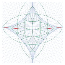
Grid lines of constant β (in blue) and ω (in green) are given in Fig. 17. These constitute an orthogonal coordinate system: the grid lines intersect at right angles. The principal sections of the ellipsoid, defined by X = 0 and Z = 0 are shown in red. The third principal section, Y = 0, is covered by the lines β = ±90° and ω = 0° or ±180°. These lines meet at four umbilical points (two of which are visible in this figure) where the principal radii of curvature are equal. Here and in the other figures in this section the parameters of the ellipsoid are a:b:c = 1.01:1:0.8, and it is viewed in an orthographic projection from a point above φ = 40°, λ = 30°.

The grid lines of the ellipsoidal coordinates may be interpreted in three different ways:

1. They are "lines of curvature" on the ellipsoid: they are parallel to the directions of principal curvature ( Monge 1796 ).
2. They are also intersections of the ellipsoid with confocal systems of hyperboloids of one and two sheets ( Dupin 1813 , Part 5 ).
3. Finally they are geodesic ellipses and hyperbolas defined using two adjacent umbilical points ( Hilbert & Cohn-Vossen 1952 , p. 188 ). For example, the lines of constant β in Fig. 17 can be generated with the familiar string construction for ellipses with the ends of the string pinned to the two umbilical points.

Jacobi's solution

Jacobi showed that the geodesic equations, expressed in ellipsoidal coordinates, are separable. Here is how he recounted his discovery to his friend and neighbor Bessel ( Jacobi 1839 , Letter to Bessel),

The day before yesterday, I reduced to quadrature the problem of geodesic lines on an ellipsoid with three unequal axes. They are the simplest formulas in the world, Abelian integrals, which become the well known elliptic integrals if 2 axes are set equal.

Königsberg, 28th Dec. '38.

The solution given by Jacobi ( Jacobi 1839 )( Jacobi 1866 , §28) is

${\displaystyle {\begin{aligned}\delta &=\int {\frac {{\sqrt {b^{2}\sin ^{2}\beta +c^{2}\cos ^{2}\beta }}\,d\beta }{{\sqrt {a^{2}-b^{2}\sin ^{2}\beta -c^{2}\cos ^{2}\beta }}{\sqrt {{\bigl (}b^{2}-c^{2}{\bigr )}\cos ^{2}\beta -\gamma }}}}\\[6pt]&\quad -\int {\frac {{\sqrt {a^{2}\sin ^{2}\omega +b^{2}\cos ^{2}\omega }}\,d\omega }{{\sqrt {a^{2}\sin ^{2}\omega +b^{2}\cos ^{2}\omega -c^{2}}}{\sqrt {{\bigl (}a^{2}-b^{2}{\bigr )}\sin ^{2}\omega +\gamma }}}}.\end{aligned}}}$

As Jacobi notes "a function of the angle β equals a function of the angle ω. These two functions are just Abelian integrals..." Two constants δ and γ appear in the solution. Typically δ is zero if the lower limits of the integrals are taken to be the starting point of the geodesic and the direction of the geodesics is determined by γ. However, for geodesics that start at an umbilical points, we have γ = 0 and δ determines the direction at the umbilical point. The constant γ may be expressed as

${\displaystyle \gamma ={\bigl (}b^{2}-c^{2}{\bigr )}\cos ^{2}\beta \sin ^{2}\alpha -{\bigl (}a^{2}-b^{2}{\bigl )}\sin ^{2}\omega \cos ^{2}\alpha ,}$

where α is the angle the geodesic makes with lines of constant ω. In the limit b→a, this reduces to sinα cosβ = const., the familiar Clairaut relation. A derivation of Jacobi's result is given by Darboux (1894 , §§583–584 ); he gives the solution found by Liouville (1846) for general quadratic surfaces.

Survey of triaxial geodesics

Circumpolar geodesics, ω₁ = 0°, α₁ = 90°.

Fig. 18. β₁ = 45.1°.

Fig. 19. β₁ = 87.48°.

On a triaxial ellipsoid, there are only three simple closed geodesics, the three principal sections of the ellipsoid given by X = 0, Y = 0, and Z = 0. ^[7] To survey the other geodesics, it is convenient to consider geodesics that intersect the middle principal section, Y = 0, at right angles. Such geodesics are shown in Figs. 18–22, which use the same ellipsoid parameters and the same viewing direction as Fig. 17. In addition, the three principal ellipses are shown in red in each of these figures.

If the starting point is β₁∈ (−90°, 90°), ω₁ = 0, and α₁ = 90°, then γ> 0 and the geodesic encircles the ellipsoid in a "circumpolar" sense. The geodesic oscillates north and south of the equator; on each oscillation it completes slightly less than a full circuit around the ellipsoid resulting, in the typical case, in the geodesic filling the area bounded by the two latitude lines β = ±β₁. Two examples are given in Figs. 18 and 19. Figure 18 shows practically the same behavior as for an oblate ellipsoid of revolution (because a≈b); compare to Fig. 9. However, if the starting point is at a higher latitude (Fig. 18) the distortions resulting from a≠b are evident. All tangents to a circumpolar geodesic touch the confocal single-sheeted hyperboloid which intersects the ellipsoid at β = β₁( Chasles 1846 )( Hilbert & Cohn-Vossen 1952 , pp. 223–224 ).

Transpolar geodesics, β₁ = 90°, α₁ = 180°.

Fig. 20. ω₁ = 39.9°.

Fig. 21. ω₁ = 9.966°.

If the starting point is β₁ = 90°, ω₁∈ (0°, 180°), and α₁ = 180°, then γ< 0 and the geodesic encircles the ellipsoid in a "transpolar" sense. The geodesic oscillates east and west of the ellipse X = 0; on each oscillation it completes slightly more than a full circuit around the ellipsoid. In the typical case, this results in the geodesic filling the area bounded by the two longitude lines ω = ω₁ and ω = 180° −ω₁. If a = b, all meridians are geodesics; the effect of a≠b causes such geodesics to oscillate east and west. Two examples are given in Figs. 20 and 21. The constriction of the geodesic near the pole disappears in the limit b→c; in this case, the ellipsoid becomes a prolate ellipsoid and Fig. 20 would resemble Fig. 10 (rotated on its side). All tangents to a transpolar geodesic touch the confocal double-sheeted hyperboloid which intersects the ellipsoid at ω = ω₁.

Fig. 22. An umbilical geodesic, β₁ = 90°, ω₁ = 0°, α₁ = 135°.

If the starting point is β₁ = 90°, ω₁ = 0° (an umbilical point), and α₁ = 135° (the geodesic leaves the ellipse Y = 0 at right angles), then γ = 0 and the geodesic repeatedly intersects the opposite umbilical point and returns to its starting point. However, on each circuit the angle at which it intersects Y = 0 becomes closer to 0° or 180° so that asymptotically the geodesic lies on the ellipse Y = 0( Hart 1849 )( Arnold 1989 , p. 265 ), as shown in Fig. 22. A single geodesic does not fill an area on the ellipsoid. All tangents to umbilical geodesics touch the confocal hyperbola that intersects the ellipsoid at the umbilic points.

Umbilical geodesic enjoy several interesting properties.

• Through any point on the ellipsoid, there are two umbilical geodesics.
• The geodesic distance between opposite umbilical points is the same regardless of the initial direction of the geodesic.
• Whereas the closed geodesics on the ellipses X = 0 and Z = 0 are stable (a geodesic initially close to and nearly parallel to the ellipse remains close to the ellipse), the closed geodesic on the ellipse Y = 0, which goes through all 4 umbilical points, is exponentially unstable. If it is perturbed, it will swing out of the plane Y = 0 and flip around before returning to close to the plane. (This behavior may repeat depending on the nature of the initial perturbation.)

If the starting point A of a geodesic is not an umbilical point, its envelope is an astroid with two cusps lying on β = −β₁ and the other two on ω = ω₁ + π. The cut locus for A is the portion of the line β = −β₁ between the cusps.

Applications

The direct and inverse geodesic problems no longer play the central role in geodesy that they once did. Instead of solving adjustment of geodetic networks as a two-dimensional problem in spheroidal trigonometry, these problems are now solved by three-dimensional methods ( Vincenty & Bowring 1978 ). Nevertheless, terrestrial geodesics still play an important role in several areas:

• for measuring distances and areas in geographic information systems;
• the definition of maritime boundaries ( UNCLOS 2006 );
• in the rules of the Federal Aviation Administration for area navigation ( RNAV 2007 );
• the method of measuring distances in the FAI Sporting Code ( FAI 2018 ).
• help Muslims find their direction toward Mecca

By the principle of least action, many problems in physics can be formulated as a variational problem similar to that for geodesics. Indeed, the geodesic problem is equivalent to the motion of a particle constrained to move on the surface, but otherwise subject to no forces ( Laplace 1799a )( Hilbert & Cohn-Vossen 1952 , p. 222 ). For this reason, geodesics on simple surfaces such as ellipsoids of revolution or triaxial ellipsoids are frequently used as "test cases" for exploring new methods. Examples include:

• the development of elliptic integrals ( Legendre 1811 ) and elliptic functions ( Weierstrass 1861 );
• the development of differential geometry ( Gauss 1828 )( Christoffel 1869 );
• methods for solving systems of differential equations by a change of independent variables ( Jacobi 1839 );
• the study of caustics ( Jacobi 1891 );
• investigations into the number and stability of periodic orbits ( Poincaré 1905 );
• in the limit c→ 0, geodesics on a triaxial ellipsoid reduce to a case of dynamical billiards;
• extensions to an arbitrary number of dimensions ( Knörrer 1980 );
• geodesic flow on a surface ( Berger 2010 , Chap. 12).

See also

• Earth section paths
• Figure of the Earth
• Geographical distance
• Great-circle navigation
• Great ellipse
• Geodesic
• Geodesy
• Map projection
  • Map projection of the triaxial ellipsoid
• Meridian arc
• Rhumb line
• Vincenty's formulae

Notes

1. Here α₂ is the forward azimuth at B. Some authors calculate the back azimuth instead; this is given by α₂±π.
2. Laplace (1799a) showed that a particle constrained to move on a surface but otherwise subject to no forces moves along a geodesic for that surface. Thus, Clairaut's relation is just a consequence of conservation of angular momentum for a particle on a surface of revolution.
3. Bagratuni (1962, §17) uses the term "coefficient of convergence of ordinates" for the geodesic scale.
4. This section is adapted from the documentation for GeographicLib (Karney 2015, Geodesics on a triaxial ellipsoid)
5. This notation for the semi-axes is incompatible with that used in the previous section on ellipsoids of revolution in which a and b stood for the equatorial radius and polar semi-axis. Thus the corresponding inequalities are a = a≥b> 0 for an oblate ellipsoid and b≥a = a> 0 for a prolate ellipsoid.
6. The limit b→c gives a prolate ellipsoid with ω playing the role of the parametric latitude.
7. If c⁄a<1⁄2, there are other simple closed geodesics similar to those shown in Figs. 11 and 12 (Klingenberg 1982, §3.5.19).

References

• Arnold, V. I. (1989). Mathematical Methods of Classical Mechanics . Translated by Vogtmann, K.; Weinstein, A. (2nd ed.). Springer-Verlag. ISBN   978-0-387-96890-2. OCLC   4037141.
• Bagratuni, G. V. (1967) [1962]. Course in Spheroidal Geodesy. doi:10.5281/zenodo.32371. OCLC   6150611. Translation from Russian of Курс сфероидической геодезии (Moscow, 1962) by U.S. Air Force (FTD-MT-64-390)
• Berger, M. (2010). Geometry Revealed. Translated by Senechal, L. J. Springer. doi:10.1007/978-3-540-70997-8. ISBN   978-3-540-70996-1.
• Bessel, F. W. (2010) [1825]. "The calculation of longitude and latitude from geodesic measurements". Astronomische Nachrichten. 331 (8). Translated by Karney, C. F. F.; Deakin, R. E.: 852–861. arXiv: 0908.1824 . Bibcode:2010AN....331..852K. doi:10.1002/asna.201011352. S2CID   118760590. English translation of Astron. Nachr.4, 241–254 (1825). Errata.
• Bliss, G. A. (1916). "Jacobi's condition for problems of the calculus of variations in parametric form". Transactions of the American Mathematical Society. 17 (2): 195–206. doi: 10.1090/S0002-9947-1916-1501037-4 .
• Bomford, G. (1952). Geodesy. Oxford: Clarendon. OCLC   1396190.
• Borre, K.; Strang, W. G. (2012). "11, Geometry of the Ellipsoid" (PDF). Algorithms for Global Positioning. Wellesley-Cambridge Press. ISBN   978-0-9802327-3-8. OCLC   795014501.
• Cayley, A. (1870). "On the geodesic lines on an oblate spheroid". Philosophical Magazine. 4th series. 40 (268): 329–340. doi:10.1080/14786447008640411.
• Chasles, M. (1846). "Sur les lignes géodésiques et les lignes de courbure des surfaces du second degré" [Geodesic lines and the lines of curvature of the surfaces of the second degree]. Journal de Mathématiques Pures et Appliquées (in French). 11: 5–20. PDF.
• Christoffel, E. B. (1869). "Allgemeine Theorie der geodätischen Dreiecke" [General theory of geodesic triangles]. Abhandlungen Königlichen Akademie der Wissenschaft zu Berlin (in German): 119–176.
• Clairaut, A. C. (1735). "Détermination géometrique de la perpendiculaire à la méridienne tracée par M. Cassini" [Geometrical determination of the perpendicular to the meridian drawn by Jacques Cassini]. Mémoires de l'Académie Royale des Sciences de Paris 1733 (in French): 406–416.
• Danielsen, J. S. (1989). "The Area under the Geodesic". Survey Review. 30 (232): 61–66. doi:10.1179/003962689791474267.
• Darboux, J. G. (1894). Leçons sur la théorie générale des surfaces [Lessons on the general theory of surfaces] (in French). Vol. 3. Paris: Gauthier-Villars. OCLC   8566228.
• Dupin, P. C. F. (1813). Développements de Géométrie [Developments in geometry] (in French). Paris: Courcier. OCLC   560800801.
• Ehlert, D. (1993). Methoden der ellipsoidischen Dreiecksberechnung[Methods for ellipsoidal triangulation] (Technical report). Reihe B: Angewandte Geodäsie, Heft Nr. 292 (in German). Deutsche Geodätische Kommission. OCLC   257615376.
• Euler, L. (1755). "Élémens de la trigonométrie sphéroïdique tirés de la méthode des plus grands et plus petits" [Elements of spheroidal trigonometry taken from the method of maxima and minima]. Mémoires de l'Académie Royale des Sciences de Berlin 1753 (in French). 9: 258–293. Figures.
• FAI (2018). "Section 8.2.3". FAI Sporting Code (PDF) (Technical report). Lausanne, Switzerland: Fédération Aéronautique Internationale.
• Forsyth, A. R. (1927). Calculus of Variations. Cambridge Univ. Press. ISBN   978-1-107-64083-2. OCLC   250050479.
• Gan'shin, V. V. (1969) [1967]. Geometry of the Earth Ellipsoid. Translated by Willis, J. M. St. Louis: Aeronautical Chart and Information Center. doi:10.5281/zenodo.32854. OCLC   493553. Translation from Russian of Геометрия земного эллипсоида (Moscow, 1967).
• Gauss, C. F. (1902) [1828]. General Investigations of Curved Surfaces of 1827 and 1825. Translated by Morehead, J. C.; Hiltebeitel, A. M. Princeton Univ. Lib. OCLC   7824448. PDF. English translation of Disquisitiones generales circa superficies curvas (Dieterich, Göttingen, 1828).
• Hart, A. S. (1849). "Geometrical demonstration of some properties of geodesic lines". Cambridge and Dublin Mathematical Journal. 4: 80–84.
• Helmert, F. R. (1964) [1880]. Mathematical and Physical Theories of Higher Geodesy. Vol. 1. St. Louis: Aeronautical Chart and Information Center. doi:10.5281/zenodo.32050. OCLC   17273288. English translation of Die Mathematischen und Physikalischen Theorieen der Höheren Geodäsie, Vol. 1 (Teubner, Leipzig, 1880).
• Hilbert, D.; Cohn-Vossen, S. (1952). Geometry and the Imagination . Translated by Nemenyi, P. New York: Chelsea. ISBN   9780828400879. OCLC   301610346.
• Hutton, C. (1811). A Course of Mathematics in Three Volumes Composed for the Use of the Royal Military Academy. Vol. 3. London: F. C. and J. Rivington. OCLC   18031510.
• Jacobi, C. G. J. (1837). "Zur Theorie der Variations-Rechnung und der Differential-Gleichungen" [The theory of the calculus of variations and of differential equations]. Journal für die Reine und Angewandte Mathematik (in German). 1837 (17): 68–82. doi:10.1515/crll.1837.17.68. S2CID   119469290.
• Jacobi, C. G. J. (1839). "Note von der geodätischen Linie auf einem Ellipsoid und den verschiedenen Anwendungen einer merkwürdigen analytischen Substitution" [The geodesic on an ellipsoid and various applications of a remarkable analytical substitution]. Journal für die Reine und Angewandte Mathematik (in German). 1839 (19): 309–313. doi:10.1515/crll.1839.19.309. S2CID   121670851. Letter to Bessel, Dec. 28, 1838. French translation (1841).
• Jacobi, C. G. J. (2009) [1866]. A. Clebsch (ed.). Lectures on Dynamics. Translated by Balagangadharan, K. New Delhi: Hindustan Book Agency. ISBN   978-81-85931-91-3. MR   2569315. OCLC   440645889. English translation of Vorlesungen über Dynamik (Reimer, Berlin, 1866). Errata.
• Jacobi, C. G. J. (1891). "Über die Curve, welche alle von einem Punkte ausgehenden geodätischen Linien eines Rotationsellipsoides berührt" [The envelope of geodesic lines emanating from a single point on an ellipsoid]. In K. T. W. Weierstrass (ed.). Jacobi's Gesammelte Werke (in German). Vol. 7. Berlin: Reimer. pp. 72–87. OCLC   630416023. Op. post., completed by F. H. A. Wangerin. PDF.
• Jekeli, C. (2012), Geometric Reference Systems in Geodesy, Ohio State Univ., hdl:1811/51274
• Jordan, W.; Eggert, O. (1962) [1941]. Handbook of Geodesy. Vol. 3. Translated by Carta, M. W. Washington, DC: Army Map Service. Bibcode:1962hage.book.....J. doi:10.5281/zenodo.35316. OCLC   34429043. English translation of Handbuch der Vermessungskunde, 8th edition (Metzler, Stuttgart, 1941).
• Karney, C. F. F. (2013). "Algorithms for geodesics". Journal of Geodesy. 87 (1): 43–55. arXiv: 1109.4448 . Bibcode:2013JGeod..87...43K. doi: 10.1007/s00190-012-0578-z . Addenda.
• Karney, C. F. F. (2015). "GeographicLib". Version 1.44.
• Karney, C. F. F. (2024). "Geodesics on an arbitrary ellipsoid of revolution". Journal of Geodesy. 98 (1): 4:1–14. arXiv: 2208.00492 . doi: 10.1007/s00190-023-01813-2 .
• Klingenberg, W. P. A. (1982). Riemannian Geometry. de Gruyer. ISBN   978-3-11-008673-7. MR   0666697. OCLC   8476832.
• Knörrer, H. (1980). "Geodesics on the ellipsoid". Inventiones Mathematicae. 59 (2): 119–143. Bibcode:1980InMat..59..119K. doi:10.1007/BF01390041. S2CID   118792545.
• Krakiwsky, E. J.; Thomson, D. B. (1974), Geodetic position computations (PDF), Dept. of Geodesy and Geomatics Engineering, Lecture Notes, Fredericton, N.B.: Univ. of New Brunswick, Bibcode:1974gpc..book.....K
• Laplace, P. S. (1829) [1799a]. "Book 1, §8.". Treatise on Celestial Mechanics. Vol. 1. Translated by Bowditch, N. Boston: Hillard, Gray, Little, & Wilkins. OCLC   1294937.
• Laplace, P. S. (1799b). Traité de Mécanique Céleste [Treatise on Celestial Mechanics] (in French). Vol. 2. Paris: Crapelet. p. 112. OCLC   25448952.
• Legendre, A. M. (1806). "Analyse des triangles tracées sur la surface d'un sphéroïde" [Analysis of spheroidal triangles]. Mémoires de l'Institut National de France (in French) (1st semester): 130–161.
• Legendre, A. M. (1811). Exercices de Calcul Intégral sur Divers Ordres de Transcendantes et sur les Quadratures [Exercises in Integral Calculus] (in French). Paris: Courcier. OCLC   312469983.
• Leick, A.; Rapoport, L.; Tatarnikov, D. (2015). GPS Satellite Surveying (4th ed.). Wiley. ISBN   978-1-119-01828-5.
• Liouville, J. (1846). "Sur quelques cas particuliers où les équations du mouvement d'un point matériel peuvent s'intégrer" [On special cases where the equations of motion of a point particle can be integrated]. Journal de Mathématiques Pures et Appliquées (in French). 11: 345–378. PDF
• Lyusternik, L. (1964). Shortest Paths: Variational Problems. Popular Lectures in Mathematics. Vol. 13. Translated by Collins, P.; Brown, R. B. New York: Macmillan. MR   0178386. OCLC   1048605. Translation from Russian of Кратчайшие Линии: Вариационные Задачи (Moscow, 1955).
• Monge, G. (1850) [1796]. "Sur les lignes de courbure de la surface de l'ellipsoïde" [On the lines of curvature on the surface of the ellipsoid]. In J. Liouville (ed.). Application de l'Analyse à la Géometrie (in French) (5th ed.). Paris: Bachelier. pp. 139–160. OCLC   2829112. (Fig. 1–2, Fig. 3–4). 1796 edition (Fig. 1–2, Fig. 3–4). PDF Figures.
• National Geodetic Survey (2012). "Geodesic Utilities: Inverse and Forward". Version 3.0.
• Newton, I. (1848) [1687]. "Book 3, Proposition 19, Problem 3". The Mathematical Principles of Natural Philosophy. Translated by Motte, A. New York: Adee. pp. 405–409. English translation of Philosophiæ Naturalis Principia Mathematica . Liber Tertius, Prop. XIX. Prob. II. pp. 422–424.
• Oriani, B. (1806). "Elementi di trigonometria sferoidica, Pt. 1" [Elements of spheroidal trigonometry]. Memorie dell'Istituto Nazionale Italiano (in Italian). 1 (1): 118–198.
• Oriani, B. (1808). "Elementi di trigonometria sferoidica, Pt. 2" [Elements of spheroidal trigonometry]. Memorie dell'Istituto Nazionale Italiano (in Italian). 2 (1): 1–58.
• Oriani, B. (1810). "Elementi di trigonometria sferoidica, Pt. 3" [Elements of spheroidal trigonometry]. Memorie dell'Istituto Nazionale Italiano (in Italian). 2 (2): 1–58.
• Poincaré, H. (1905). "Sur les lignes géodésiques des surfaces convexes" [Geodesics lines on convex surfaces]. Transactions of the American Mathematical Society (in French). 6 (3): 237–274. doi:10.2307/1986219. JSTOR   1986219.
• Rainsford, H. F. (1955). "Long geodesics on the ellipsoid". Bulletin Géodésique . 37 (1): 12–22. Bibcode:1955BGeod..29...12R. doi:10.1007/BF02527187. S2CID   122111614.
• Rapp, R. H. (1991), Geometric geodesy, part I, Ohio State Univ., hdl:1811/24333
• Rapp, R. H. (1993), Geometric geodesy, part II, Ohio State Univ., hdl:1811/24409
• RNAV (2007). "Appendix 2.". Order 8260.54A, The United States Standard for Area Navigation (PDF) (Technical report). Washington, D.C.: U.S. Federal Aviation Administration.
• Sjöberg, L. E. (2006). "Determination of areas on the plane, sphere and ellipsoid". Survey Review. 38 (301): 583–593. doi:10.1179/003962606780732100.
• UNCLOS (2006). A Manual on Technical Aspects of the United Nations Convention on the Law of the Sea, 1982 (PDF) (Technical report) (4th ed.). Monaco: International Hydrographic Bureau. Archived from the original (PDF) on 2013-05-24. Retrieved 2013-08-15.
• Vincenty, T. (1975). "Direct and inverse solutions of geodesics on the ellipsoid with application of nested equations" (PDF). Survey Review. 23 (176): 88–93. Bibcode:1975SurRv..23...88V. doi:10.1179/sre.1975.23.176.88. Addendum: Survey Review 23 (180): 294 (1976).
• Vincenty, T.; Bowring, B. R. (1978). Application of three-dimensional geodesy to adjustments of horizontal networks (PDF) (Technical report). NOAA. NOS NGS-13.
• Weierstrass, K. T. W. (1861). "Über die geodätischen Linien auf dem dreiaxigen Ellipsoid" [Geodesic lines on a triaxial ellipsoid]. Monatsberichte der Königlichen Akademie der Wissenschaft zu Berlin (in German): 986–997.

External links

• Online geodesic bibliography of books and articles on geodesics on ellipsoids.
• Test set for geodesics, a set of 500000 geodesics for the WGS84 ellipsoid, computed using high-precision arithmetic.
• NGS tool implementing Vincenty (1975).
• geod(1), man page for the PROJ utility for geodesic calculations.
• GeographicLib implementation of Karney (2013).
• Drawing geodesics on Google Maps.