Haldane's dilemma

Last updated December 16, 2024

Haldane's dilemma, also known as the waiting time problem,^[1] is a limit on the speed of beneficial evolution, calculated by J. B. S. Haldane in 1957. Before the invention of DNA sequencing technologies, it was not known how much polymorphism DNA harbored, although alloenzymes (variant forms of an enzyme which differ structurally but not functionally from other alloenzymes coded for by different alleles at the same locus) were beginning to make it clear that substantial polymorphism existed. This was puzzling because the amount of polymorphism known to exist seemed to exceed the theoretical limits that Haldane calculated, that is, the limits imposed if polymorphisms present in the population generally influence an organism's fitness. Motoo Kimura's landmark paper on neutral theory in 1968^[2] built on Haldane's work to suggest that most molecular evolution is neutral, resolving the dilemma. Although neutral evolution remains the consensus theory among modern biologists,^[3] and thus Kimura's resolution of Haldane's dilemma is widely regarded as correct, some biologists argue that adaptive evolution explains a large fraction of substitutions in protein coding sequence,^[4] and they propose alternative solutions to Haldane's dilemma.

Substitution cost

In the introduction to The Cost of Natural Selection Haldane writes that it is difficult for breeders to simultaneously select all the desired qualities, partly because the required genes may not be found together in the stock; but, he writes,^[5]

especially in slowly breeding animals such as cattle, one cannot cull even half the females, even though only one in a hundred of them combines the various qualities desired.^[5]

That is, the problem for the cattle breeder is that keeping only the specimens with the desired qualities will lower the reproductive capability too much to keep a useful breeding stock.

Haldane states that this same problem arises with respect to natural selection. Characters that are positively correlated at one time may be negatively correlated at a later time, so simultaneous optimization of more than one character is a problem also in nature. And, as Haldane writes^[5]

[i]n this paper I shall try to make quantitative the fairly obvious statement that natural selection cannot occur with great intensity for a number of characters at once unless they happen to be controlled by the same genes.^[5]

In faster breeding species there is less of a problem. Haldane mentions the peppered moth, Biston betularia, whose variation in pigmentation is determined by several alleles at a single gene.^[5]^[6] One of these alleles, "C", is dominant to all the others, and any CC or Cx moths are dark (where "x" is any other allele). Another allele, "c", is recessive to all the others, and cc moths are light. Against the originally pale lichens the darker moths were easier for birds to pick out, but in areas, where pollution has darkened the lichens, the cc moths had become rare. Haldane mentions that in a single day the frequency of cc moths might be halved.

Another potential problem is that if "ten other independently inherited characters had been subject to selection of the same intensity as that for colour, only $(1/2)^{10}$ , or one in 1024, of the original genotype would have survived." The species would most likely have become extinct; but it might well survive ten other selective periods of comparable selectivity, if they happened in different centuries.^[5]

Selection intensity

Haldane proceeds to define the intensity of selection regarding "juvenile survival" (that is, survival to reproductive age) as $I=\ln(s_{0}/S)$ , where $s_{0}$ is the proportion of those with the optimal genotype (or genotypes) that survive to reproduce, and $S$ is the proportion of the entire population that similarly so survive. The proportion for the entire population that die without reproducing is thus $1-S$ , and this would have been $1-s_{0}$ if all genotypes had survived as well as the optimal. Hence $s_{0}-S$ is the proportion of "genetic" deaths due to selection. As Haldane mentions, if $s_{0}\approx S$ , then $I\approx s_{0}-S$ .^[7]

The cost

Haldane writes

I shall investigate the following case mathematically. A population is in equilibrium under selection and mutation. One or more genes are rare because their appearance by mutation is balanced by natural selection. A sudden change occurs in the environment, for example, pollution by smoke, a change of climate, the introduction of a new food source, predator, or pathogen, and above all migration to a new habitat. It will be shown later that the general conclusions are not affected if the change is slow. The species is less adapted to the new environment, and its reproductive capacity is lowered. It is gradually improved as a result of natural selection. But meanwhile, a number of deaths, or their equivalents in lowered fertility, have occurred. If selection at the $i^{th}$ selected locus is responsible for $d_{i}$ of these deaths in any generation the reproductive capacity of the species will be $\prod \left(1-d_{i}\right)$ of that of the optimal genotype, or $\exp \left(-\sum d_{i}\right)$ nearly, if every $d_{i}$ is small. Thus the intensity of selection approximates to $\sum d_{i}$ .^[5]

Comparing to the above, we have that $d_{i}=s_{0i}-S$ , if we say that $s_{0i}$ is the quotient of deaths for the $i^{th}$ selected locus and $S$ is again the quotient of deaths for the entire population.

The problem statement is therefore that the alleles in question are not particularly beneficial under the previous circumstances; but a change in environment favors these genes by natural selection. The individuals without the genes are therefore disfavored, and the favorable genes spread in the population by the death (or lowered fertility) of the individuals without the genes. Note that Haldane's model as stated here allows for more than one gene to move towards fixation at a time; but each such will add to the cost of substitution.

The total cost of substitution of the $i^{th}$ gene is the sum $D_{i}$ of all values of $d_{i}$ over all generations of selection; that is, until fixation of the gene. Haldane states that he will show that $D_{i}$ depends mainly on $p_{0}$ , the small frequency of the gene in question, as selection begins – that is, at the time that the environmental change occurs (or begins to occur).^[5]

A mathematical model of the cost of diploids

Let A and a be two alleles with frequencies $p_{n}$ and $q_{n}$ in the $n^{\mbox{th}}$ generation. Their relative fitness is given by^[5]

Genotype AA Aa aa
Frequency $p_{n}^{2}$ $2p_{n}q_{n}$ $q_{n}^{2}$
Fitness 1 $1-\lambda K$ $1-K$

where 0 ≤ $K$ ≤ 1, and 0 ≤ λ ≤ 1.

If λ = 0, then Aa has the same fitness as AA, e.g. if Aa is phenotypically equivalent with AA (A dominant), and if λ = 1, then Aa has the same fitness as aa, e.g. if Aa is phenotypically equivalent with aa (A recessive). In general λ indicates how close in fitness Aa is to aa.

The fraction of selective deaths in the $n^{\mbox{th}}$ generation then is

d_{n}=2\lambda Kp_{n}q_{n}+Kq_{n}^{2}=Kq_{n}[2\lambda +(1-2\lambda )q_{n}]

and the total number of deaths is the population size multiplied by

D=K\sum _{0}^{\infty }q_{n}\;[2\lambda +(1-2\lambda )q_{n}].

Important number 300

Haldane approximates the above equation by taking the continuum limit of the above equation.^[5] This is done by multiplying and dividing it by dq so that it is in integral form

dq_{n}=-Kp_{n}q_{n}[\lambda +(1-2\lambda )q_{n}]

substituting q=1-p, the cost (given by the total number of deaths, 'D', required to make a substitution) is given by

D=\int _{0}^{q_{_{0}}}{\frac {[2\lambda +(1-2\lambda )q]}{(1-q)[\lambda +(1-2\lambda )q]}}dq={\frac {1}{1-\lambda }}\int _{0}^{q_{_{0}}}\left[{\frac {1}{1-q}}+{\frac {\lambda (1-2\lambda )}{\lambda +(1-2\lambda )q}}\right]dq.

Assuming λ < 1, this gives

D={\frac {1}{1-\lambda }}\left[-{\mbox{ln }}p_{0}+\lambda {\mbox{ ln }}\left({\frac {1-\lambda -(1-2\lambda )p_{0}}{\lambda }}\right)\right]\approx {\frac {1}{1-\lambda }}\left[-{\mbox{ln }}p_{0}+\lambda {\mbox{ ln }}\left({\frac {1-\lambda }{\lambda }}\right)\right]

where the last approximation assumes $p_{0}$ to be small.

If λ = 1, then we have

D=\int _{0}^{q_{_{0}}}{\frac {2-q}{(1-q)^{2}}}dq=\int _{0}^{q_{_{0}}}\left[{\frac {1}{1-q}}+{\frac {1}{(1-q)^{2}}}\right]dq=p_{0}^{-1}-{\mbox{ ln }}p_{0}+O(\lambda K).

In his discussion Haldane writes that the substitution cost, if it is paid by juvenile deaths, "usually involves a number of deaths equal to about 10 or 20 times the number in a generation" – the minimum being the population size (= "the number in a generation") and rarely being 100 times that number. Haldane assumes 30 to be the mean value.^[5]

Assuming substitution of genes to take place slowly, one gene at a time over n generations, the fitness of the species will fall below the optimum (achieved when the substitution is complete) by a factor of about 30/n, so long as this is small – small enough to prevent extinction. Haldane doubts that high intensities – such as in the case of the peppered moth – have occurred frequently and estimates that a value of n = 300 is a probable number of generations. This gives a selection intensity of $I=30/300=0.1$ .

Haldane then continues:^[5]

The number of loci in a vertebrate species has been estimated at about 40,000. 'Good' species, even when closely related, may differ at several thousand loci, even if the differences at most of them are very slight. But it takes as many deaths, or their equivalents, to replace a gene by one producing a barely distinguishable phenotype as by one producing a very different one. If two species differ at 1000 loci, and the mean rate of gene substitution, as has been suggested, is one per 300 generations, it will take 300,000 generations to generate an interspecific difference. It may take a good deal more, for if an allele a1 is replaced by a10, the population may pass through stages where the commonest genotype is a1a1, a2a2, a3a3, and so on, successively, the various alleles in turn giving maximal fitness in the existing environment and the residual environment.^[5]

The number 300 of generations is a conservative estimate for a slowly evolving species not at the brink of extinction by Haldane's calculation. For a difference of at least 1,000 genes, 300,000 generations might be needed – maybe more, if some gene runs through more than one optimisation.

Origin of the term "Haldane's dilemma"

Apparently the first use of the term "Haldane's dilemma" was by paleontologist Leigh Van Valen in his 1963 paper "Haldane's Dilemma, Evolutionary Rates, and Heterosis".

Van Valen writes:^[8]

Haldane (1957 [= The Cost of Natural Selection]) drew attention to the fact that in the process of the evolutionary substitution of one allele for another, at any intensity of selection and no matter how slight the importance of the locus, a substantial number of individuals would usually be lost because they did not already possess the new allele. Kimura (1960, 1961) has referred to this loss as the substitutional (or evolutional) load, but because it necessarily involves either a completely new mutation or (more usually) previous change in the environment or the genome, I like to think of it as a dilemma for the population: for most organisms, rapid turnover in a few genes precludes rapid turnover in the others. A corollary of this is that, if an environmental change occurs that necessitates the rather rapid replacement of several genes if a population is to survive, the population becomes extinct.^[8]

That is, since a high number of deaths are required to fix one gene rapidly, and dead organisms do not reproduce, fixation of more than one gene simultaneously would conflict. Note that Haldane's model assumes independence of genes at different loci; if the selection intensity is 0.1 for each gene moving towards fixation, and there are N such genes, then the reproductive capacity of the species will be lowered to 0.9^N times the original capacity. Therefore, if it is necessary for the population to fix more than one gene, it may not have reproductive capacity to counter the deaths.

Evolution above Haldane's limit

Various models evolve at rates above Haldane's limit.

J. A. Sved^[9] showed that a threshold model of selection, where individuals with a phenotype less than the threshold die and individuals with a phenotype above the threshold are all equally fit, allows for a greater substitution rate than Haldane's model (though no obvious upper limit was found, though tentative paths to calculate one were examined e.g. the death rate). John Maynard Smith^[10] and Peter O'Donald^[11] followed on the same track.

Additionally, the effects of density-dependent processes, epistasis, and soft selective sweeps on the maximum rate of substitution have been examined.^[12]

By looking at the polymorphisms within species and divergence between species an estimate can be obtained for the fraction of substitutions that occur due to selection. This parameter is generally called alpha (hence DFE-alpha), and appears to be large in some species, although almost all approaches suggest that the human-chimp divergence was primarily neutral. However, if divergence between Drosophila species was as adaptive as the alpha parameter suggests, then it would exceed Haldane's limit.

Related Research Articles

In probability theory and statistics, the exponential distribution or negative exponential distribution is the probability distribution of the distance between events in a Poisson point process, i.e., a process in which events occur continuously and independently at a constant average rate; the distance parameter could be any meaningful mono-dimensional measure of the process, such as time between production errors, or length along a roll of fabric in the weaving manufacturing process. It is a particular case of the gamma distribution. It is the continuous analogue of the geometric distribution, and it has the key property of being memoryless. In addition to being used for the analysis of Poisson point processes it is found in various other contexts.

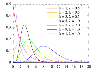
The Erlang distribution is a two-parameter family of continuous probability distributions with support $. The two parameters are:$

In probability theory and statistics, the Weibull distribution is a continuous probability distribution. It models a broad range of random variables, largely in the nature of a time to failure or time between events. Examples are maximum one-day rainfalls and the time a user spends on a web page.

In probability theory and statistics, the gamma distribution is a versatile two-parameter family of continuous probability distributions. The exponential distribution, Erlang distribution, and chi-squared distribution are special cases of the gamma distribution. There are two equivalent parameterizations in common use:

With a shape parameter $α$ and a scale parameter $θ$
With a shape parameter $and a rate parameter ⁠ ⁠$

Allele frequency, or gene frequency, is the relative frequency of an allele at a particular locus in a population, expressed as a fraction or percentage. Specifically, it is the fraction of all chromosomes in the population that carry that allele over the total population or sample size. Microevolution is the change in allele frequencies that occurs over time within a population.

Quantitative genetics is the study of quantitative traits, which are phenotypes that vary continuously—such as height or mass—as opposed to phenotypes and gene-products that are discretely identifiable—such as eye-colour, or the presence of a particular biochemical.

<span class="mw-page-title-main">Partition function (statistical mechanics)</span> Function in thermodynamics and statistical physics

In physics, a partition function describes the statistical properties of a system in thermodynamic equilibrium. Partition functions are functions of the thermodynamic state variables, such as the temperature and volume. Most of the aggregate thermodynamic variables of the system, such as the total energy, free energy, entropy, and pressure, can be expressed in terms of the partition function or its derivatives. The partition function is dimensionless.

<span class="mw-page-title-main">Exponential decay</span> Decrease in value at a rate proportional to the current value

A quantity is subject to exponential decay if it decreases at a rate proportional to its current value. Symbolically, this process can be expressed by the following differential equation, where $N$ is the quantity and $λ$ (lambda) is a positive rate called the exponential decay constant, disintegration constant, rate constant, or transformation constant:

Population dynamics is the type of mathematics used to model and study the size and age composition of populations as dynamical systems.

Variational Bayesian methods are a family of techniques for approximating intractable integrals arising in Bayesian inference and machine learning. They are typically used in complex statistical models consisting of observed variables as well as unknown parameters and latent variables, with various sorts of relationships among the three types of random variables, as might be described by a graphical model. As typical in Bayesian inference, the parameters and latent variables are grouped together as "unobserved variables". Variational Bayesian methods are primarily used for two purposes:

To provide an analytical approximation to the posterior probability of the unobserved variables, in order to do statistical inference over these variables.
To derive a lower bound for the marginal likelihood of the observed data. This is typically used for performing model selection, the general idea being that a higher marginal likelihood for a given model indicates a better fit of the data by that model and hence a greater probability that the model in question was the one that generated the data.

Mutation–selection balance is an equilibrium in the number of deleterious alleles in a population that occurs when the rate at which deleterious alleles are created by mutation equals the rate at which deleterious alleles are eliminated by selection. The majority of genetic mutations are neutral or deleterious; beneficial mutations are relatively rare. The resulting influx of deleterious mutations into a population over time is counteracted by negative selection, which acts to purge deleterious mutations. Setting aside other factors, the equilibrium number of deleterious alleles is then determined by a balance between the deleterious mutation rate and the rate at which selection purges those mutations.

In statistics and information theory, a maximum entropy probability distribution has entropy that is at least as great as that of all other members of a specified class of probability distributions. According to the principle of maximum entropy, if nothing is known about a distribution except that it belongs to a certain class, then the distribution with the largest entropy should be chosen as the least-informative default. The motivation is twofold: first, maximizing entropy minimizes the amount of prior information built into the distribution; second, many physical systems tend to move towards maximal entropy configurations over time.

The principle of detailed balance can be used in kinetic systems which are decomposed into elementary processes. It states that at equilibrium, each elementary process is in equilibrium with its reverse process.

Genetic distance is a measure of the genetic divergence between species or between populations within a species, whether the distance measures time from common ancestor or degree of differentiation. Populations with many similar alleles have small genetic distances. This indicates that they are closely related and have a recent common ancestor.

Plasma parameters define various characteristics of a plasma, an electrically conductive collection of charged and neutral particles of various species that responds collectively to electromagnetic forces. Such particle systems can be studied statistically, i.e., their behaviour can be described based on a limited number of global parameters instead of tracking each particle separately.

Covariance matrix adaptation evolution strategy (CMA-ES) is a particular kind of strategy for numerical optimization. Evolution strategies (ES) are stochastic, derivative-free methods for numerical optimization of non-linear or non-convex continuous optimization problems. They belong to the class of evolutionary algorithms and evolutionary computation. An evolutionary algorithm is broadly based on the principle of biological evolution, namely the repeated interplay of variation and selection: in each generation (iteration) new individuals are generated by variation of the current parental individuals, usually in a stochastic way. Then, some individuals are selected to become the parents in the next generation based on their fitness or objective function value $. Like this, individuals with better and better -values are generated over the generation sequence.$

Formalized by John Tukey, the Tukey lambda distribution is a continuous, symmetric probability distribution defined in terms of its quantile function. It is typically used to identify an appropriate distribution and not used in statistical models directly.

In probability theory and statistics, the Conway–Maxwell–Poisson distribution is a discrete probability distribution named after Richard W. Conway, William L. Maxwell, and Siméon Denis Poisson that generalizes the Poisson distribution by adding a parameter to model overdispersion and underdispersion. It is a member of the exponential family, has the Poisson distribution and geometric distribution as special cases and the Bernoulli distribution as a limiting case.

In probability theory and statistics, the Poisson distribution is a discrete probability distribution that expresses the probability of a given number of events occurring in a fixed interval of time if these events occur with a known constant mean rate and independently of the time since the last event. It can also be used for the number of events in other types of intervals than time, and in dimension greater than 1.

<span class="mw-page-title-main">Lomax distribution</span> Heavy-tail probability distribution

The Lomax distribution, conditionally also called the Pareto Type II distribution, is a heavy-tail probability distribution used in business, economics, actuarial science, queueing theory and Internet traffic modeling. It is named after K. S. Lomax. It is essentially a Pareto distribution that has been shifted so that its support begins at zero.

References

↑ Sanford J, Brewer W, Smith F, Baumgardner J (September 2015). "The waiting time problem in a model hominin population". Theoretical Biology & Medical Modelling. 12 (1): 18. doi: 10.1186/s12976-015-0016-z . PMC 4573302 . PMID 26376851.
↑ Kimura M (February 1968). "Evolutionary rate at the molecular level". Nature. 217 (5129): 624–6. Bibcode:1968Natur.217..624K. doi:10.1038/217624a0. PMID 5637732. S2CID 4161261.
↑ Jensen JD, Payseur BA, Stephan W, Aquadro CF, Lynch M, Charlesworth D, Charlesworth B (January 2019). "The importance of the Neutral Theory in 1968 and 50 years on: A response to Kern and Hahn 2018". Evolution; International Journal of Organic Evolution. 73 (1): 111–114. doi:10.1111/evo.13650. PMC 6496948 . PMID 30460993.
↑ Kern AD, Hahn MW (June 2018). "The Neutral Theory in Light of Natural Selection". Molecular Biology and Evolution. 35 (6): 1366–1371. doi:10.1093/molbev/msy092. PMC 5967545 . PMID 29722831.
1 2 3 4 5 6 7 8 9 10 11 12 13 14 Haldane JB. "The Cost of Natural Selection" (PDF). J. Genet. 55 (511–524): 1957.
↑ Majerus ME (1998). Melanism: Evolution in Action . New York: Oxford University Press.
↑ See Haldane.^[5] If $a=1-s_{0}$ and $b=1-S$ , then $I=\ln(1-a)-\ln(1-b)\approx -a+b=s_{0}-S$ .
1 2 Van Valen L (1963). "Haldane's Dilemma, evolutionary rates, and heterosis". Am. Nat. 47 (894): 185–190. Bibcode:1963ANat...97..185V. doi:10.1086/282267. S2CID 222327449.
↑ Sved JA (June 1968). "Possible Rates of Gene Substitution in Evolution". American Naturalist. 102 (925): 283–93. Bibcode:1968ANat..102..283S. doi:10.1086/282542. S2CID 84618125.
↑ Maynard Smith J (September 1968). ""Haldane's dilemma" and the rate of evolution". Nature. 219 (5159): 1114–6. Bibcode:1968Natur.219.1114S. doi:10.1038/2191114a0. PMID 5675622. S2CID 864709.
↑ O'Donald P (March 1969). ""Haldane's dilemma" and the Rate of Natural Selection". Nature. 221 (5183): 815–6. Bibcode:1969Natur.221..815O. doi:10.1038/221815a0. PMID 5765051. S2CID 4288246.
↑ Nunney L (January 2003). "The cost of natural selection revisited" (PDF). Annales Zoologici Fennici. 40. Finnish Zoological and Botanical Publishing Board.: 185–194.