Harmonic mean p-value

Last updated

The harmonic mean p-value [1] [2] [3] (HMP) is a statistical technique for addressing the multiple comparisons problem that controls the strong-sense family-wise error rate [2] (this claim has been disputed [4] ). It improves on the power of Bonferroni correction by performing combined tests, i.e. by testing whether groups of p-values are statistically significant, like Fisher's method. [5] However, it avoids the restrictive assumption that the p-values are independent, unlike Fisher's method. [2] [3] Consequently, it controls the false positive rate when tests are dependent, at the expense of less power (i.e. a higher false negative rate) when tests are independent. [2] Besides providing an alternative to approaches such as Bonferroni correction that controls the stringent family-wise error rate, it also provides an alternative to the widely-used Benjamini-Hochberg procedure (BH) for controlling the less-stringent false discovery rate. [6] This is because the power of the HMP to detect significant groups of hypotheses is greater than the power of BH to detect significant individual hypotheses. [2]

Contents

There are two versions of the technique: (i) direct interpretation of the HMP as an approximate p-value and (ii) a procedure for transforming the HMP into an asymptotically exact p-value. The approach provides a multilevel test procedure in which the smallest groups of p-values that are statistically significant may be sought.

Direct interpretation of the harmonic mean p-value

The weighted harmonic mean of p-values is defined as

where are weights that must sum to one, i.e. . Equal weights may be chosen, in which case .

In general, interpreting the HMP directly as a p-value is anti-conservative, meaning that the false positive rate is higher than expected. However, as the HMP becomes smaller, under certain assumptions, the discrepancy decreases, so that direct interpretation of significance achieves a false positive rate close to that implied for sufficiently small values (e.g. ). [2]

The HMP is never anti-conservative by more than a factor of for small , or for large . [3] However, these bounds represent worst case scenarios under arbitrary dependence that are likely to be conservative in practice. Rather than applying these bounds, asymptotically exact p-values can be produced by transforming the HMP.

Asymptotically exact harmonic mean p-value procedure

Generalized central limit theorem shows that an asymptotically exact p-value, , can be computed from the HMP, , using the formula [2]

Subject to the assumptions of generalized central limit theorem, this transformed p-value becomes exact as the number of tests, , becomes large. The computation uses the Landau distribution, whose density function can be written

The test is implemented by the p.hmp command of the harmonicmeanp R package; a tutorial is available online.

Equivalently, one can compare the HMP to a table of critical values (Table 1). The table illustrates that the smaller the false positive rate, and the smaller the number of tests, the closer the critical value is to the false positive rate.

Table 1. Critical values for the HMP for varying numbers of tests and false positive rates . [2]
100.0400.00940.00099
1000.0360.00920.00099
1,0000.0340.00900.00099
10,0000.0310.00880.00098
100,0000.0290.00860.00098
1,000,0000.0270.00840.00098
10,000,0000.0260.00830.00098
100,000,0000.0240.00810.00098
1,000,000,0000.0230.00800.00097

Multiple testing via the multilevel test procedure

If the HMP is significant at some level for a group of p-values, one may search all subsets of the p-values for the smallest significant group, while maintaining the strong-sense family-wise error rate. [2] Formally, this constitutes a closed-testing procedure. [7]

When is small (e.g. ), the following multilevel test based on direct interpretation of the HMP controls the strong-sense family-wise error rate at level approximately

  1. Define the HMP of any subset of the p-values to be
  2. Reject the null hypothesis that none of the p-values in subset are significant if , where . (Recall that, by definition, .)


An asymptotically exact version of the above replaces in step 2 with

where gives the number of p-values, not just those in subset . [8]

Since direct interpretation of the HMP is faster, a two-pass procedure may be used to identify subsets of p-values that are likely to be significant using direct interpretation, subject to confirmation using the asymptotically exact formula.

Properties of the HMP

The HMP has a range of properties that arise from generalized central limit theorem. [2] It is:

When the HMP is not significant, neither is any subset of the constituent tests. Conversely, when the multilevel test deems a subset of p-values to be significant, the HMP for all the p-values combined is likely to be significant; this is certain when the HMP is interpreted directly. When the goal is to assess the significance of individualp-values, so that combined tests concerning groups of p-values are of no interest, the HMP is equivalent to the Bonferroni procedure but subject to the more stringent significance threshold (Table 1).

The HMP assumes the individual p-values have (not necessarily independent) standard uniform distributions when their null hypotheses are true. Large numbers of underpowered tests can therefore harm the power of the HMP.

While the choice of weights is unimportant for the validity of the HMP under the null hypothesis, the weights influence the power of the procedure. Supplementary Methods §5C of [2] and an online tutorial consider the issue in more detail.

Bayesian interpretations of the HMP

The HMP was conceived by analogy to Bayesian model averaging and can be interpreted as inversely proportional to a model-averaged Bayes factor when combining p-values from likelihood ratio tests. [1] [2]

The harmonic mean rule-of-thumb

I. J. Good reported an empirical relationship between the Bayes factor and the p-value from a likelihood ratio test. [1] For a null hypothesis nested in a more general alternative hypothesis he observed that often,

where denotes the Bayes factor in favour of versus Extrapolating, he proposed a rule of thumb in which the HMP is taken to be inversely proportional to the model-averaged Bayes factor for a collection of tests with common null hypothesis:

For Good, his rule-of-thumb supported an interchangeability between Bayesian and classical approaches to hypothesis testing. [9] [10] [11] [12] [13]

Bayesian calibration of p-values

If the distributions of the p-values under the alternative hypotheses follow Beta distributions with parameters , a form considered by Sellke, Bayarri and Berger, [14] then the inverse proportionality between the model-averaged Bayes factor and the HMP can be formalized as [2] [15]

where

The approximation works best for well-powered tests ().

The harmonic mean p-value as a bound on the Bayes factor

For likelihood ratio tests with exactly two degrees of freedom, Wilks' theorem implies that , where is the maximized likelihood ratio in favour of alternative hypothesis and therefore , where is the weighted mean maximized likelihood ratio, using weights Since is an upper bound on the Bayes factor, , then is an upper bound on the model-averaged Bayes factor:

While the equivalence holds only for two degrees of freedom, the relationship between and and therefore behaves similarly for other degrees of freedom. [2] Under the assumption that the distributions of the p-values under the alternative hypotheses follow Beta distributions with parameters and that the weights the HMP provides a tighter upper bound on the model-averaged Bayes factor:

a result that again reproduces the inverse proportionality of Good's empirical relationship. [16]

Related Research Articles

<span class="mw-page-title-main">Normal distribution</span> Probability distribution

In statistics, a normal distribution or Gaussian distribution is a type of continuous probability distribution for a real-valued random variable. The general form of its probability density function is

In probability theory, the central limit theorem (CLT) establishes that, in many situations, when independent random variables are summed up, their properly normalized sum tends toward a normal distribution even if the original variables themselves are not normally distributed.

In statistics, the likelihood-ratio test assesses the goodness of fit of two competing statistical models based on the ratio of their likelihoods, specifically one found by maximization over the entire parameter space and another found after imposing some constraint. If the constraint is supported by the observed data, the two likelihoods should not differ by more than sampling error. Thus the likelihood-ratio test tests whether this ratio is significantly different from one, or equivalently whether its natural logarithm is significantly different from zero.

<span class="mw-page-title-main">Fourier transform</span> Mathematical transform that expresses a function of time as a function of frequency

A Fourier transform (FT) is a mathematical transform that decomposes functions into frequency components, which are represented by the output of the transform as a function of frequency. Most commonly functions of time or space are transformed, which will output a function depending on temporal frequency or spatial frequency respectively. That process is also called analysis. An example application would be decomposing the waveform of a musical chord into terms of the intensity of its constituent pitches. The term Fourier transform refers to both the frequency domain representation and the mathematical operation that associates the frequency domain representation to a function of space or time.

In probability theory, Chebyshev's inequality guarantees that, for a wide class of probability distributions, no more than a certain fraction of values can be more than a certain distance from the mean. Specifically, no more than 1/k2 of the distribution's values can be k or more standard deviations away from the mean. The rule is often called Chebyshev's theorem, about the range of standard deviations around the mean, in statistics. The inequality has great utility because it can be applied to any probability distribution in which the mean and variance are defined. For example, it can be used to prove the weak law of large numbers.

In probability theory and statistics, a Gaussian process is a stochastic process, such that every finite collection of those random variables has a multivariate normal distribution, i.e. every finite linear combination of them is normally distributed. The distribution of a Gaussian process is the joint distribution of all those random variables, and as such, it is a distribution over functions with a continuous domain, e.g. time or space.

In physics and probability theory, Mean-field theory (MFT) or Self-consistent field theory studies the behavior of high-dimensional random (stochastic) models by studying a simpler model that approximates the original by averaging over degrees of freedom. Such models consider many individual components that interact with each other.

In physics, the Hamilton–Jacobi equation, named after William Rowan Hamilton and Carl Gustav Jacob Jacobi, is an alternative formulation of classical mechanics, equivalent to other formulations such as Newton's laws of motion, Lagrangian mechanics and Hamiltonian mechanics. The Hamilton–Jacobi equation is particularly useful in identifying conserved quantities for mechanical systems, which may be possible even when the mechanical problem itself cannot be solved completely.

In statistics, G-tests are likelihood-ratio or maximum likelihood statistical significance tests that are increasingly being used in situations where chi-squared tests were previously recommended.

In mathematics, the Riesz–Thorin theorem, often referred to as the Riesz–Thorin interpolation theorem or the Riesz–Thorin convexity theorem, is a result about interpolation of operators. It is named after Marcel Riesz and his student G. Olof Thorin.

In probability theory and statistics, the generalized extreme value (GEV) distribution is a family of continuous probability distributions developed within extreme value theory to combine the Gumbel, Fréchet and Weibull families also known as type I, II and III extreme value distributions. By the extreme value theorem the GEV distribution is the only possible limit distribution of properly normalized maxima of a sequence of independent and identically distributed random variables. Note that a limit distribution needs to exist, which requires regularity conditions on the tail of the distribution. Despite this, the GEV distribution is often used as an approximation to model the maxima of long (finite) sequences of random variables.

In statistics and probability theory, a point process or point field is a collection of mathematical points randomly located on a mathematical space such as the real line or Euclidean space. Point processes can be used for spatial data analysis, which is of interest in such diverse disciplines as forestry, plant ecology, epidemiology, geography, seismology, materials science, astronomy, telecommunications, computational neuroscience, economics and others.

In statistics, family-wise error rate (FWER) is the probability of making one or more false discoveries, or type I errors when performing multiple hypotheses tests.

In directional statistics, the von Mises–Fisher distribution, is a probability distribution on the -sphere in . If the distribution reduces to the von Mises distribution on the circle.

Expected shortfall (ES) is a risk measure—a concept used in the field of financial risk measurement to evaluate the market risk or credit risk of a portfolio. The "expected shortfall at q% level" is the expected return on the portfolio in the worst of cases. ES is an alternative to value at risk that is more sensitive to the shape of the tail of the loss distribution.

<span class="mw-page-title-main">Generalized Pareto distribution</span> Family of probability distributions often used to model tails or extreme values

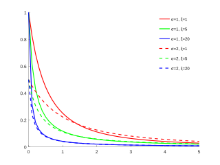
In statistics, the generalized Pareto distribution (GPD) is a family of continuous probability distributions. It is often used to model the tails of another distribution. It is specified by three parameters: location , scale , and shape . Sometimes it is specified by only scale and shape and sometimes only by its shape parameter. Some references give the shape parameter as .

Linear Programming Boosting (LPBoost) is a supervised classifier from the boosting family of classifiers. LPBoost maximizes a margin between training samples of different classes and hence also belongs to the class of margin-maximizing supervised classification algorithms. Consider a classification function

In mathematics — specifically, in stochastic analysis — the infinitesimal generator of a Feller process is a Fourier multiplier operator that encodes a great deal of information about the process. The generator is used in evolution equations such as the Kolmogorov backward equation ; its L2 Hermitian adjoint is used in evolution equations such as the Fokker–Planck equation.

<span class="mw-page-title-main">Dirichlet kernel</span>

In mathematical analysis, the Dirichlet kernel, named after the German mathematician Peter Gustav Lejeune Dirichlet, is the collection of periodic functions defined as

In optimal transport, a branch of mathematics, polar factorization of vector fields is a basic result due to Brenier (1987), with antecedents of Knott-Smith (1984) and Rachev (1985), that generalizes many existing results among which are the polar decomposition of real matrices, and the rearrangement of real-valued functions.

References

  1. 1 2 3 Good, I J (1958). "Significance tests in parallel and in series". Journal of the American Statistical Association. 53 (284): 799–813. doi:10.1080/01621459.1958.10501480. JSTOR   2281953.
  2. 1 2 3 4 5 6 7 8 9 10 11 12 13 14 Wilson, D J (2019). "The harmonic mean p-value for combining dependent tests". Proceedings of the National Academy of Sciences USA. 116 (4): 1195–1200. doi: 10.1073/pnas.1814092116 . PMC   6347718 . PMID   30610179.
  3. 1 2 3 Vovk, Vladimir; Wang, Ruodu (April 25, 2019). "Combining p-values via averaging" (PDF). Algorithmic Learning in a Random World.
  4. Goeman, Jelle J.; Rosenblatt, Jonathan D.; Nichols, Thomas E. (2019-11-19). "The harmonic mean p-value: Strong versus weak control, and the assumption of independence". Proceedings of the National Academy of Sciences. 116 (47): 23382–23383. doi: 10.1073/pnas.1909339116 . ISSN   0027-8424. PMC   6876242 . PMID   31662466.
  5. Fisher, R A (1934). Statistical Methods for Research Workers (5th ed.). Edinburgh, UK: Oliver and Boyd.
  6. Benjamini Y, Hochberg Y (1995). "Controlling the false discovery rate: A practical and powerful approach to multiple testing". Journal of the Royal Statistical Society. Series B (Methodological). 57 (1): 289–300. doi:10.1111/j.2517-6161.1995.tb02031.x. JSTOR   2346101.
  7. Marcus R, Eric P, Gabriel KR (1976). "On closed testing procedures with special reference to ordered analysis of variance". Biometrika. 63 (3): 655–660. doi:10.1093/biomet/63.3.655. JSTOR   2335748.
  8. Wilson, Daniel J (August 17, 2019). "Updated correction to "The harmonic mean p-value for combining independent tests"" (PDF).
  9. Good, I J (1984). "C192. One tail versus two-tails, and the harmonic-mean rule of thumb". Journal of Statistical Computation and Simulation. 19 (2): 174–176. doi:10.1080/00949658408810727.
  10. Good, I J (1984). "C193. Paired versus unpaired comparisons and the harmonic-mean rule of thumb". Journal of Statistical Computation and Simulation. 19 (2): 176–177. doi:10.1080/00949658408810728.
  11. Good, I J (1984). "C213. A sharpening of the harmonic-mean rule of thumb for combining tests "in parallel"". Journal of Statistical Computation and Simulation. 20 (2): 173–176. doi:10.1080/00949658408810770.
  12. Good, I J (1984). "C214. The harmonic-mean rule of thumb: Some classes of applications". Journal of Statistical Computation and Simulation. 20 (2): 176–179. doi:10.1080/00949658408810771.
  13. Good, Irving John. (2009). Good thinking : the foundations of probability and its applications. Dover Publications. ISBN   9780486474380. OCLC   319491702.
  14. Sellke, Thomas; Bayarri, M. J; Berger, James O (2001). "Calibration of p Values for Testing Precise Null Hypotheses". The American Statistician. 55 (1): 62–71. doi:10.1198/000313001300339950. ISSN   0003-1305. S2CID   396772.
  15. Wilson, D J (2019). "Reply to Held: When is a harmonic mean p-value a Bayes factor?" (PDF). Proceedings of the National Academy of Sciences USA. 116 (13): 5857–5858. doi: 10.1073/pnas.1902157116 . PMC   6442550 . PMID   30890643.
  16. Held, L (2019). "On the Bayesian interpretation of the harmonic mean p-value". Proceedings of the National Academy of Sciences USA. 116 (13): 5855–5856. doi: 10.1073/pnas.1900671116 . PMC   6442579 . PMID   30890644.