Hydrodynamic stability

Last updated
A simple diagram of the transition from a stable flow to a turbulent flow. a) stable, b) turbulent Laminar and turbulent flows.svg
A simple diagram of the transition from a stable flow to a turbulent flow. a) stable, b) turbulent

In fluid dynamics, hydrodynamic stability is the field which analyses the stability and the onset of instability of fluid flows. The study of hydrodynamic stability aims to find out if a given flow is stable or unstable, and if so, how these instabilities will cause the development of turbulence. [1] The foundations of hydrodynamic stability, both theoretical and experimental, were laid most notably by Helmholtz, Kelvin, Rayleigh and Reynolds during the nineteenth century. [1] These foundations have given many useful tools to study hydrodynamic stability. These include Reynolds number, the Euler equations, and the Navier–Stokes equations. When studying flow stability it is useful to understand more simplistic systems, e.g. incompressible and inviscid fluids which can then be developed further onto more complex flows. [1] Since the 1980s, more computational methods are being used to model and analyse the more complex flows.

Contents

Stable and unstable flows

To distinguish between the different states of fluid flow one must consider how the fluid reacts to a disturbance in the initial state. [2] These disturbances will relate to the initial properties of the system, such as velocity, pressure, and density. James Clerk Maxwell expressed the qualitative concept of stable and unstable flow nicely when he said: [1]

"when an infinitely small variation of the present state will alter only by an infinitely small quantity the state at some future time, the condition of the system, whether at rest or in motion, is said to be stable but when an infinitely small variation in the present state may bring about a finite difference in the state of the system in a finite time, the system is said to be unstable."

That means that for a stable flow, any infinitely small variation, which is considered a disturbance, will not have any noticeable effect on the initial state of the system and will eventually die down in time. [2] For a fluid flow to be considered stable it must be stable with respect to every possible disturbance. This implies that there exists no mode of disturbance for which it is unstable. [1]

On the other hand, for an unstable flow, any variations will have some noticeable effect on the state of the system which would then cause the disturbance to grow in amplitude in such a way that the system progressively departs from the initial state and never returns to it. [2] This means that there is at least one mode of disturbance with respect to which the flow is unstable, and the disturbance will therefore distort the existing force equilibrium. [3]

Determining flow stability

Reynolds number

A key tool used to determine the stability of a flow is the Reynolds number (Re), first put forward by George Gabriel Stokes at the start of the 1850s. Associated with Osborne Reynolds who further developed the idea in the early 1880s, this dimensionless number gives the ratio of inertial terms and viscous terms. [4] In a physical sense, this number is a ratio of the forces which are due to the momentum of the fluid (inertial terms), and the forces which arise from the relative motion of the different layers of a flowing fluid (viscous terms). The equation for this is [2]

where

  • is the density
  • is the velocity of the fluid flow
  • is the dynamic viscosity, i.e., a measure of the fluids' resistance to shearing flows
  • is the characteristic length of the system
  • is the kinematic viscosity – it measures the ratio of dynamic viscosity to the density of the fluid

The Reynolds number is useful because it can provide cut off points for when flow is stable or unstable, namely the Critical Reynolds number . As it increases, the amplitude of a disturbance which could then lead to instability gets smaller. [1] At high Reynolds numbers it is agreed that fluid flows will be unstable. High Reynolds number can be achieved in several ways, e.g. if is a small value or if and are high values. [2] This means that instabilities will arise almost immediately and the flow will become unstable or turbulent. [1]

In order to analytically find the stability of fluid flows, it is useful to note that hydrodynamic stability has a lot in common with stability in other fields, such as magnetohydrodynamics, plasma physics and elasticity; although the physics is different in each case, the mathematics and the techniques used are similar. The essential problem is modeled by nonlinear partial differential equations and the stability of known steady and unsteady solutions are examined. [1] The governing equations for almost all hydrodynamic stability problems are the Navier–Stokes equation and the continuity equation. The Navier–Stokes equation is given by: [1]

where

Here is being used as an operator acting on the velocity field on the left hand side of the equation and then acting on the pressure on the right hand side.

and the continuity equation is given by:

where is the material derivative of the density.

Once again is being used as an operator on and is calculating the divergence of the velocity.

But if the fluid being considered is incompressible, which means the density is constant, then and hence:

The assumption that a flow is incompressible is a good one and applies to most fluids travelling at most speeds. It is assumptions of this form that will help to simplify the Navier–Stokes equation into differential equations, like Euler's equation, which are easier to work with.

Euler's equation

If one considers a flow which is inviscid, this is where the viscous forces are small and can therefore be neglected in the calculations, then one arrives at Euler's equations:

Although in this case we have assumed an inviscid fluid this assumption does not hold for flows where there is a boundary. The presence of a boundary causes some viscosity at the boundary layer which cannot be neglected and one arrives back at the Navier–Stokes equation. Finding the solutions to these governing equations under different circumstances and determining their stability is the fundamental principle in determining the stability of the fluid flow itself.

Linear stability analysis

To determine whether the flow is stable or unstable, one often employs the method of linear stability analysis. In this type of analysis, the governing equations and boundary conditions are linearized. This is based on the fact that the concept of 'stable' or 'unstable' is based on an infinitely small disturbance. For such disturbances, it is reasonable to assume that disturbances of different wavelengths evolve independently. (A nonlinear governing equation will allow disturbances of different wavelengths to interact with each other.)

Analysing flow stability

Bifurcation theory

Bifurcation theory is a useful way to study the stability of a given flow, with the changes that occur in the structure of a given system. Hydrodynamic stability is a series of differential equations and their solutions. A bifurcation occurs when a small change in the parameters of the system causes a qualitative change in its behavior,. [1] The parameter that is being changed in the case of hydrodynamic stability is the Reynolds number. It can be shown that the occurrence of bifurcations falls in line with the occurrence of instabilities. [1]

Laboratory and computational experiments

Laboratory experiments are a very useful way of gaining information about a given flow without having to use more complex mathematical techniques. Sometimes physically seeing the change in the flow over time is just as useful as a numerical approach and any findings from these experiments can be related back to the underlying theory. Experimental analysis is also useful because it allows one to vary the governing parameters very easily and their effects will be visible.

When dealing with more complicated mathematical theories such as Bifurcation theory and Weakly nonlinear theory, numerically solving such problems becomes very difficult and time-consuming but with the help of computers this process becomes much easier and quicker. Since the 1980s computational analysis has become more and more useful, the improvement of algorithms which can solve the governing equations, such as the Navier–Stokes equation, means that they can be integrated more accurately for various types of flow.

Applications

Kelvin–Helmholtz instability

This is an image, captured in San Francisco, which shows the "ocean wave" like pattern associated with the Kelvin-Helmholtz instability forming in clouds. Kelvin Helmholz wave clouds.jpg
This is an image, captured in San Francisco, which shows the "ocean wave" like pattern associated with the Kelvin–Helmholtz instability forming in clouds.

The Kelvin–Helmholtz instability (KHI) is an application of hydrodynamic stability that can be seen in nature. It occurs when there are two fluids flowing at different velocities. The difference in velocity of the fluids causes a shear velocity at the interface of the two layers. [3] The shear velocity of one fluid moving induces a shear stress on the other which, if greater than the restraining surface tension, then results in an instability along the interface between them. [3] This motion causes the appearance of a series of overturning ocean waves, a characteristic of the Kelvin–Helmholtz instability. Indeed, the apparent ocean wave-like nature is an example of vortex formation, which are formed when a fluid is rotating about some axis, and is often associated with this phenomenon.

The Kelvin–Helmholtz instability can be seen in the bands in planetary atmospheres such as Saturn and Jupiter, for example in the giant red spot vortex. In the atmosphere surrounding the giant red spot there is the biggest example of KHI that is known of and is caused by the shear force at the interface of the different layers of Jupiter's atmosphere. There have been many images captured where the ocean-wave like characteristics discussed earlier can be seen clearly, with as many as 4 shear layers visible. [5]

Weather satellites take advantage of this instability to measure wind speeds over large bodies of water. Waves are generated by the wind, which shears the water at the interface between it and the surrounding air. The computers on board the satellites determine the roughness of the ocean by measuring the wave height. This is done by using radar, where a radio signal is transmitted to the surface and the delay from the reflected signal is recorded, known as the "time of flight". From this meteorologists are able to understand the movement of clouds and the expected air turbulence near them.

Rayleigh–Taylor instability

This is a 2D model of the Rayleigh-Taylor instability occurring between two fluids. In this model the red fluid - initially on top, and afterwards below - represents a more dense fluid and the blue fluid represents one which is less dense. Model of the initiation of termination of a Rayleigh-Taylor instability in 2D.gif
This is a 2D model of the Rayleigh–Taylor instability occurring between two fluids. In this model the red fluid – initially on top, and afterwards below – represents a more dense fluid and the blue fluid represents one which is less dense.

The Rayleigh–Taylor instability is another application of hydrodynamic stability and also occurs between two fluids but this time the densities of the fluids are different. [6] Due to the difference in densities, the two fluids will try to reduce their combined potential energy. [7] The less dense fluid will do this by trying to force its way upwards, and the more dense fluid will try to force its way downwards. [6] Therefore, there are two possibilities: if the lighter fluid is on top the interface is said to be stable, but if the heavier fluid is on top, then the equilibrium of the system is unstable to any disturbances of the interface. If this is the case then both fluids will begin to mix. [6] Once a small amount of heavier fluid is displaced downwards with an equal volume of lighter fluid upwards, the potential energy is now lower than the initial state, [7] therefore the disturbance will grow and lead to the turbulent flow associated with Rayleigh–Taylor instabilities. [6]

This phenomenon can be seen in interstellar gas, such as the Crab Nebula. It is pushed out of the Galactic plane by magnetic fields and cosmic rays and then becomes Rayleigh–Taylor unstable if it is pushed past its normal scale height. [6] This instability also explains the mushroom cloud which forms in processes such as volcanic eruptions and atomic bombs.

Rayleigh–Taylor instability has a big effect on the Earth's climate. Winds that come from the coast of Greenland and Iceland cause evaporation of the ocean surface over which they pass, increasing the salinity of the ocean water near the surface, and making the water near the surface denser. This then generates plumes which drive the ocean currents. This process acts as a heat pump, transporting warm equatorial water North. Without the ocean overturning, Northern Europe would likely face drastic drops in temperature. [6]

See also

Notes

  1. 1 2 3 4 5 6 7 8 9 10 11 See Drazin (2002), Introduction to hydrodynamic stability
  2. 1 2 3 4 5 See Chandrasekhar (1961) "Hydrodynamic and Hydromagnetic stability"
  3. 1 2 3 See V.Shankar – Department of Chemical Engineering IIT Kanpur (2014), "Introduction to hydrodynamic stability"
  4. See J.Happel, H.Brenner (2009, 2nd edition) "Low Reynolds number hydrodynamics"
  5. See the Astrophysical journal letters, volume 729, no. 1 (2009), "Magnetic Kelvin–Helmholtz instability at the Sun"
  6. 1 2 3 4 5 6 See J.Oakley (2004), "Rayleigh–Taylor instability notes"
  7. 1 2 See A.W.Cook, D.Youngs (2009), "Rayleigh–Taylor instability and mixing"

Related Research Articles

<span class="mw-page-title-main">Fluid dynamics</span> Aspects of fluid mechanics involving flow

In physics, physical chemistry and engineering, fluid dynamics is a subdiscipline of fluid mechanics that describes the flow of fluids—liquids and gases. It has several subdisciplines, including aerodynamics and hydrodynamics. Fluid dynamics has a wide range of applications, including calculating forces and moments on aircraft, determining the mass flow rate of petroleum through pipelines, predicting weather patterns, understanding nebulae in interstellar space and modelling fission weapon detonation.

<span class="mw-page-title-main">Navier–Stokes equations</span> Equations describing the motion of viscous fluid substances

The Navier–Stokes equations are partial differential equations which describe the motion of viscous fluid substances, named after French engineer and physicist Claude-Louis Navier and Irish physicist and mathematician George Gabriel Stokes. They were developed over several decades of progressively building the theories, from 1822 (Navier) to 1842-1850 (Stokes).

The vorticity equation of fluid dynamics describes the evolution of the vorticity ω of a particle of a fluid as it moves with its flow; that is, the local rotation of the fluid. The governing equation is:

In fluid dynamics, Stokes' law is an empirical law for the frictional force – also called drag force – exerted on spherical objects with very small Reynolds numbers in a viscous fluid. It was derived by George Gabriel Stokes in 1851 by solving the Stokes flow limit for small Reynolds numbers of the Navier–Stokes equations.

In fluid mechanics or more generally continuum mechanics, incompressible flow refers to a flow in which the material density is constant within a fluid parcel—an infinitesimal volume that moves with the flow velocity. An equivalent statement that implies incompressibility is that the divergence of the flow velocity is zero.

<span class="mw-page-title-main">D'Alembert's paradox</span>

In fluid dynamics, d'Alembert's paradox is a contradiction reached in 1752 by French mathematician Jean le Rond d'Alembert. D'Alembert proved that – for incompressible and inviscid potential flow – the drag force is zero on a body moving with constant velocity relative to the fluid. Zero drag is in direct contradiction to the observation of substantial drag on bodies moving relative to fluids, such as air and water; especially at high velocities corresponding with high Reynolds numbers. It is a particular example of the reversibility paradox.

<span class="mw-page-title-main">Rayleigh–Taylor instability</span> Unstable behavior of two contacting fluids of different densities

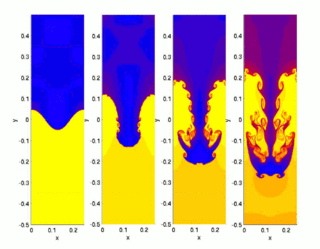
The Rayleigh–Taylor instability, or RT instability, is an instability of an interface between two fluids of different densities which occurs when the lighter fluid is pushing the heavier fluid. Examples include the behavior of water suspended above oil in the gravity of Earth, mushroom clouds like those from volcanic eruptions and atmospheric nuclear explosions, supernova explosions in which expanding core gas is accelerated into denser shell gas, instabilities in plasma fusion reactors and inertial confinement fusion.

<span class="mw-page-title-main">Stokes flow</span> Type of fluid flow

Stokes flow, also named creeping flow or creeping motion, is a type of fluid flow where advective inertial forces are small compared with viscous forces. The Reynolds number is low, i.e. . This is a typical situation in flows where the fluid velocities are very slow, the viscosities are very large, or the length-scales of the flow are very small. Creeping flow was first studied to understand lubrication. In nature, this type of flow occurs in the swimming of microorganisms and sperm. In technology, it occurs in paint, MEMS devices, and in the flow of viscous polymers generally.

In fluid mechanics, potential vorticity (PV) is a quantity which is proportional to the dot product of vorticity and stratification. This quantity, following a parcel of air or water, can only be changed by diabatic or frictional processes. It is a useful concept for understanding the generation of vorticity in cyclogenesis, especially along the polar front, and in analyzing flow in the ocean.

The Orr–Sommerfeld equation, in fluid dynamics, is an eigenvalue equation describing the linear two-dimensional modes of disturbance to a viscous parallel flow. The solution to the Navier–Stokes equations for a parallel, laminar flow can become unstable if certain conditions on the flow are satisfied, and the Orr–Sommerfeld equation determines precisely what the conditions for hydrodynamic stability are.

The intent of this article is to highlight the important points of the derivation of the Navier–Stokes equations as well as its application and formulation for different families of fluids.

The Cauchy momentum equation is a vector partial differential equation put forth by Cauchy that describes the non-relativistic momentum transport in any continuum.

In a body submerged in a fluid, unsteady forces due to acceleration of that body with respect to the fluid, can be divided into two parts: the virtual mass effect and the Basset force.

In fluid dynamics, the Oseen equations describe the flow of a viscous and incompressible fluid at small Reynolds numbers, as formulated by Carl Wilhelm Oseen in 1910. Oseen flow is an improved description of these flows, as compared to Stokes flow, with the (partial) inclusion of convective acceleration.

In fluid dynamics, The projection method is an effective means of numerically solving time-dependent incompressible fluid-flow problems. It was originally introduced by Alexandre Chorin in 1967 as an efficient means of solving the incompressible Navier-Stokes equations. The key advantage of the projection method is that the computations of the velocity and the pressure fields are decoupled.

<span class="mw-page-title-main">Reynolds number</span> Ratio of inertial to viscous forces acting on a liquid

In fluid mechanics, the Reynolds number is a dimensionless quantity that helps predict fluid flow patterns in different situations by measuring the ratio between inertial and viscous forces. At low Reynolds numbers, flows tend to be dominated by laminar (sheet-like) flow, while at high Reynolds numbers, flows tend to be turbulent. The turbulence results from differences in the fluid's speed and direction, which may sometimes intersect or even move counter to the overall direction of the flow. These eddy currents begin to churn the flow, using up energy in the process, which for liquids increases the chances of cavitation.

In fluid mechanics, non-dimensionalization of the Navier–Stokes equations is the conversion of the Navier–Stokes equation to a nondimensional form. This technique can ease the analysis of the problem at hand, and reduce the number of free parameters. Small or large sizes of certain dimensionless parameters indicate the importance of certain terms in the equations for the studied flow. This may provide possibilities to neglect terms in the considered flow. Further, non-dimensionalized Navier–Stokes equations can be beneficial if one is posed with similar physical situations – that is problems where the only changes are those of the basic dimensions of the system.

The Darrieus–Landau instability or hydrodynamic instability is an instrinsic flame instability that occurs in premixed flames, caused by the density variation due to the thermal expansion of the gas produced by the combustion process. In simple terms, the stability inquires whether a steadily propagating plane sheet with a discontinuous jump in density is stable or not. It was predicted independently by Georges Jean Marie Darrieus and Lev Landau.

<span class="mw-page-title-main">Rayleigh's equation (fluid dynamics)</span>

In fluid dynamics, Rayleigh's equation or Rayleigh stability equation is a linear ordinary differential equation to study the hydrodynamic stability of a parallel, incompressible and inviscid shear flow. The equation is:

In fluid mechanics, Helmholtz minimum dissipation theorem states that the steady Stokes flow motion of an incompressible fluid has the smallest rate of dissipation than any other incompressible motion with the same velocity on the boundary. The theorem also has been studied by Diederik Korteweg in 1883 and by Lord Rayleigh in 1913.

References