IBM alignment models

Last updated

IBM alignment models are a sequence of increasingly complex models used in statistical machine translation to train a translation model and an alignment model, starting with lexical translation probabilities and moving to reordering and word duplication. [1] They underpinned the majority of statistical machine translation systems for almost twenty years starting in the early 1990s, until neural machine translation began to dominate. These models offer principled probabilistic formulation and (mostly) tractable inference. [2]

Contents

The original work on statistical machine translation at IBM proposed five models, and a model 6 was proposed later. The sequence of the six models can be summarized as:

Mathematical setup

The IBM alignment models translation as a conditional probability model. For each source-language ("foreign") sentence , we generate both a target-language ("English") sentence and an alignment . The problem then is to find a good statistical model for , the probability that we would generate English language sentence and an alignment given a foreign sentence .

The meaning of an alignment grows increasingly complicated as the model version number grew. See Model 1 for the most simple and understandable version.

Model 1

Word alignment

Given any foreign-English sentence pair , an alignment for the sentence pair is a function of type . That is, we assume that the English word at location is "explained" by the foreign word at location . For example, consider the following pair of sentences

It will surely rain tomorrow -- 明日 は きっと 雨 だ

We can align some English words to corresponding Japanese words, but not everyone:

it -> ?

will -> ?

surely -> きっと

rain -> 雨

tomorrow -> 明日

This in general happens due to the different grammar and conventions of speech in different languages. English sentences require a subject, and when there is no subject available, it uses a dummy pronoun it. Japanese verbs do not have different forms for future and present tense, and the future tense is implied by the noun 明日 (tomorrow). Conversely, the topic-marker は and the grammar word だ (roughly "to be") do not correspond to any word in the English sentence. So, we can write the alignment as

1-> 0; 2 -> 0; 3 -> 3; 4 -> 4; 5 -> 1

where 0 means that there is no corresponding alignment.

Thus, we see that the alignment function is in general a function of type .

Future models will allow one English world to be aligned with multiple foreign words.

Statistical model

Given the above definition of alignment, we can define the statistical model used by Model 1:

Together, we have the probability

IBM Model 1 uses very simplistic assumptions on the statistical model, in order to allow the following algorithm to have closed-form solution.

Learning from a corpus

If a dictionary is not provided at the start, but we have a corpus of English-foreign language pairs (without alignment information), then the model can be cast into the following form:


In this form, this is exactly the kind of problem solved by expectation–maximization algorithm. Due to the simplistic assumptions, the algorithm has a closed-form, efficiently computable solution, which is the solution to the following equations:

This can be solved by Lagrangian multipliers, then simplified. For a detailed derivation of the algorithm, see [3] chapter 4 and. [4] In short, the EM algorithm goes as follows:

INPUT. a corpus of English-foreign sentence pairs


INITIALIZE. matrix of translations probabilities .

This could either be uniform or random. It is only required that every entry is positive, and for each , the probability sums to one: .

LOOP. until converges:

where each is a normalization constant that makes sure each .

RETURN. .

In the above formula, is the Dirac delta function -- it equals 1 if the two entries are equal, and 0 otherwise. The index notation is as follows:

ranges over English-foreign sentence pairs in corpus;

ranges over words in English sentences;

ranges over words in foreign language sentences;

ranges over the entire vocabulary of English words in the corpus;

ranges over the entire vocabulary of foreign words in the corpus.

Limitations

There are several limitations to the IBM model 1. [3]

Model 2

Model 2 allows alignment to be conditional on sentence lengths. That is, we have a probability distribution , meaning "the probability that English word is aligned to foreign word , when the English sentence is of length , and the foreign sentence is of length ".

The rest of Model 1 is unchanged. With that, we have

The EM algorithm can still be solved in closed-form, giving the following algorithm:

where are still normalization factors. See section 4.4.1 [3] of for a derivation and an algorithm.

Model 3


The fertility problem is addressed in IBM Model 3. The fertility is modeled using probability distribution defined as:

For each foreign word , such distribution indicates to how many output words it usually translates. This model deals with dropping input words because it allows . But there is still an issue when adding words. For example, the English word do is often inserted when negating. This issue generates a special NULL token that can also have its fertility modeled using a conditional distribution defined as:

The number of inserted words depends on sentence length. This is why the NULL token insertion is modeled as an additional step: the fertility step. It increases the IBM Model 3 translation process to four steps:

IBM models 03.jpg

The last step is called distortion instead of alignment because it is possible to produce the same translation with the same alignment in different ways. For example, in the above example, we have another way to get the same alignment: [5]

IBM Model 3 can be mathematically expressed as:

where represents the fertility of , each source word is assigned a fertility distribution , and and refer to the absolute lengths of the target and source sentences, respectively. [6]

See section 4.4.2 [3] of for a derivation and an algorithm.

Model 4

In IBM Model 4, each word is dependent on the previously aligned word and on the word classes of the surrounding words. Some words tend to get reordered during translation more than others (e.g. adjective–noun inversion when translating Polish to English). Adjectives often get moved before the noun that precedes them. The word classes introduced in Model 4 solve this problem by conditioning the probability distributions of these classes. The result of such distribution is a lexicalized model. Such a distribution can be defined as follows:

For the initial word in the cept:

For additional words:

where and functions map words to their word classes, and and are distortion probability distributions of the words. The cept is formed by aligning each input word to at least one output word. [7]

Both Model 3 and Model 4 ignore if an input position was chosen and if the probability mass was reserved for the input positions outside the sentence boundaries. It is the reason for the probabilities of all correct alignments not sum up to unity in these two models (deficient models). [7]

Model 5

IBM Model 5 reformulates IBM Model 4 by enhancing the alignment model with more training parameters in order to overcome the model deficiency. [8] During the translation in Model 3 and Model 4 there are no heuristics that would prohibit the placement of an output word in a position already taken. In Model 5 it is important to place words only in free positions. It is done by tracking the number of free positions and allowing placement only in such positions. The distortion model is similar to IBM Model 4, but it is based on free positions. If denotes the number of free positions in the output, the IBM Model 5 distortion probabilities would be defined as: [9]

For the initial word in the cept:

For additional words:

The alignment models that use first-order dependencies like the HMM or IBM Models 4 and 5 produce better results than the other alignment methods. The main idea of HMM is to predict the distance between subsequent source language positions. On the other hand, IBM Model 4 tries to predict the distance between subsequent target language positions. Since it was expected to achieve better alignment quality when using both types of such dependencies, HMM and Model 4 were combined in a log-linear manner in Model 6 as follows: [10]

where the interpolation parameter is used in order to count the weight of Model 4 relatively to the hidden Markov model. A log-linear combination of several models can be defined as with as:

The log-linear combination is used instead of linear combination because the values are typically different in terms of their orders of magnitude for HMM and IBM Model 4. [11]

Related Research Articles

First-order logic—also known as predicate logic, quantificational logic, and first-order predicate calculus—is a collection of formal systems used in mathematics, philosophy, linguistics, and computer science. First-order logic uses quantified variables over non-logical objects, and allows the use of sentences that contain variables, so that rather than propositions such as "Socrates is a man", one can have expressions in the form "there exists x such that x is Socrates and x is a man", where "there exists" is a quantifier, while x is a variable. This distinguishes it from propositional logic, which does not use quantifiers or relations; in this sense, propositional logic is the foundation of first-order logic.

Propositional calculus is a branch of logic. It is also called propositional logic, statement logic, sentential calculus, sentential logic, or sometimes zeroth-order logic. It deals with propositions and relations between propositions, including the construction of arguments based on them. Compound propositions are formed by connecting propositions by logical connectives. Propositions that contain no logical connectives are called atomic propositions.

<span class="mw-page-title-main">Normal distribution</span> Probability distribution

In statistics, a normal distribution or Gaussian distribution is a type of continuous probability distribution for a real-valued random variable. The general form of its probability density function is

<span class="mw-page-title-main">Logistic regression</span> Statistical model for a binary dependent variable

In statistics, the logistic model is a statistical model that models the probability of an event taking place by having the log-odds for the event be a linear combination of one or more independent variables. In regression analysis, logistic regression is estimating the parameters of a logistic model. Formally, in binary logistic regression there is a single binary dependent variable, coded by an indicator variable, where the two values are labeled "0" and "1", while the independent variables can each be a binary variable or a continuous variable. The corresponding probability of the value labeled "1" can vary between 0 and 1, hence the labeling; the function that converts log-odds to probability is the logistic function, hence the name. The unit of measurement for the log-odds scale is called a logit, from logistic unit, hence the alternative names. See § Background and § Definition for formal mathematics, and § Example for a worked example.

<span class="mw-page-title-main">Path integral formulation</span> Formulation of quantum mechanics

The path integral formulation is a description in quantum mechanics that generalizes the action principle of classical mechanics. It replaces the classical notion of a single, unique classical trajectory for a system with a sum, or functional integral, over an infinity of quantum-mechanically possible trajectories to compute a quantum amplitude.

In logic, a truth function is a function that accepts truth values as input and produces a unique truth value as output. In other words: The input and output of a truth function are all truth values; a truth function will always output exactly one truth value; and inputting the same truth value(s) will always output the same truth value. The typical example is in propositional logic, wherein a compound statement is constructed using individual statements connected by logical connectives; if the truth value of the compound statement is entirely determined by the truth value(s) of the constituent statement(s), the compound statement is called a truth function, and any logical connectives used are said to be truth functional.

In the theory of stochastic processes, the Karhunen–Loève theorem, also known as the Kosambi–Karhunen–Loève theorem states that a stochastic process can be represented as an infinite linear combination of orthogonal functions, analogous to a Fourier series representation of a function on a bounded interval. The transformation is also known as Hotelling transform and eigenvector transform, and is closely related to principal component analysis (PCA) technique widely used in image processing and in data analysis in many fields.

In statistics, a mixture model is a probabilistic model for representing the presence of subpopulations within an overall population, without requiring that an observed data set should identify the sub-population to which an individual observation belongs. Formally a mixture model corresponds to the mixture distribution that represents the probability distribution of observations in the overall population. However, while problems associated with "mixture distributions" relate to deriving the properties of the overall population from those of the sub-populations, "mixture models" are used to make statistical inferences about the properties of the sub-populations given only observations on the pooled population, without sub-population identity information.

BLEU is an algorithm for evaluating the quality of text which has been machine-translated from one natural language to another. Quality is considered to be the correspondence between a machine's output and that of a human: "the closer a machine translation is to a professional human translation, the better it is" – this is the central idea behind BLEU. Invented at IBM in 2001, BLEU was one of the first metrics to claim a high correlation with human judgements of quality, and remains one of the most popular automated and inexpensive metrics.

Statistical machine translation (SMT) was a machine translation approach, that superseded the previous, rule-based approach because it required explicit description of each and every linguistic rule, which was costly, and which often did not generalize to other languages. Since 2003, the statistical approach itself has been gradually superseded by the deep learning-based neural network approach.

<span class="mw-page-title-main">Bitext word alignment</span> Identifying translation relationships among the words in a bitext

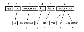
Bitext word alignment or simply word alignment is the natural language processing task of identifying translation relationships among the words in a bitext, resulting in a bipartite graph between the two sides of the bitext, with an arc between two words if and only if they are translations of one another. Word alignment is typically done after sentence alignment has already identified pairs of sentences that are translations of one another.

In information theory, perplexity is a measurement of how well a probability distribution or probability model predicts a sample. It may be used to compare probability models. A low perplexity indicates the probability distribution is good at predicting the sample. Perplexity was originally introduced in 1977 in the context of speech recognition by Frederick Jelinek, Robert Leroy Mercer, Lalit R. Bahl, and James K. Baker.

Probabilistic Computation Tree Logic (PCTL) is an extension of computation tree logic (CTL) that allows for probabilistic quantification of described properties. It has been defined in the paper by Hansson and Jonsson.

<span class="mw-page-title-main">Autoencoder</span> Neural network that learns efficient data encoding in an unsupervised manner

An autoencoder is a type of artificial neural network used to learn efficient codings of unlabeled data. An autoencoder learns two functions: an encoding function that transforms the input data, and a decoding function that recreates the input data from the encoded representation. The autoencoder learns an efficient representation (encoding) for a set of data, typically for dimensionality reduction.

In probability theory and statistics, the Dirichlet-multinomial distribution is a family of discrete multivariate probability distributions on a finite support of non-negative integers. It is also called the Dirichlet compound multinomial distribution (DCM) or multivariate Pólya distribution. It is a compound probability distribution, where a probability vector p is drawn from a Dirichlet distribution with parameter vector , and an observation drawn from a multinomial distribution with probability vector p and number of trials n. The Dirichlet parameter vector captures the prior belief about the situation and can be seen as a pseudocount: observations of each outcome that occur before the actual data is collected. The compounding corresponds to a Pólya urn scheme. It is frequently encountered in Bayesian statistics, machine learning, empirical Bayes methods and classical statistics as an overdispersed multinomial distribution.

In probability theory and statistical mechanics, the Gaussian free field (GFF) is a Gaussian random field, a central model of random surfaces (random height functions). Sheffield (2007) gives a mathematical survey of the Gaussian free field.

Least-squares support-vector machines (LS-SVM) for statistics and in statistical modeling, are least-squares versions of support-vector machines (SVM), which are a set of related supervised learning methods that analyze data and recognize patterns, and which are used for classification and regression analysis. In this version one finds the solution by solving a set of linear equations instead of a convex quadratic programming (QP) problem for classical SVMs. Least-squares SVM classifiers were proposed by Johan Suykens and Joos Vandewalle. LS-SVMs are a class of kernel-based learning methods.

Inductive probability attempts to give the probability of future events based on past events. It is the basis for inductive reasoning, and gives the mathematical basis for learning and the perception of patterns. It is a source of knowledge about the world.

Bayesian hierarchical modelling is a statistical model written in multiple levels that estimates the parameters of the posterior distribution using the Bayesian method. The sub-models combine to form the hierarchical model, and Bayes' theorem is used to integrate them with the observed data and account for all the uncertainty that is present. The result of this integration is the posterior distribution, also known as the updated probability estimate, as additional evidence on the prior distribution is acquired.

<span class="mw-page-title-main">Transformer (machine learning model)</span> Machine learning algorithm used for natural-language processing

A transformer is a deep learning architecture that relies on the parallel multi-head attention mechanism. The modern transformer was proposed in the 2017 paper titled 'Attention Is All You Need' by Ashish Vaswani et al., Google Brain team. It is notable for requiring less training time than previous recurrent neural architectures, such as long short-term memory (LSTM), and its later variation has been prevalently adopted for training large language models on large (language) datasets, such as the Wikipedia corpus and Common Crawl, by virtue of the parallelized processing of input sequence. Input text is split into n-grams encoded as tokens and each token is converted into a vector via looking up from a word embedding table. At each layer, each token is then contextualized within the scope of the context window with other (unmasked) tokens via a parallel multi-head attention mechanism allowing the signal for key tokens to be amplified and less important tokens to be diminished. Though the transformer paper was published in 2017, the softmax-based attention mechanism was proposed earlier in 2014 by Bahdanau, Cho, and Bengio for machine translation, and the Fast Weight Controller, similar to a transformer, was proposed in 1992 by Schmidhuber.

References

  1. "IBM Models". SMT Research Survey Wiki. 11 September 2015. Retrieved 26 October 2015.
  2. Yarin Gal; Phil Blunsom (12 June 2013). "A Systematic Bayesian Treatment of the IBM Alignment Models" (PDF). University of Cambridge. Archived from the original (PDF) on 4 Mar 2016. Retrieved 26 October 2015.
  3. 1 2 3 4 Koehn, Philipp (2010). "4. Word-Based Models". Statistical Machine Translation. Cambridge University Press. ISBN   978-0-521-87415-1.
  4. "CS288, Spring 2020, Lectur 05: Statistical Machine Translation" (PDF). Archived (PDF) from the original on 24 Oct 2020.
  5. Wołk K., Marasek K. (2014). Polish-English Speech Statistical Machine Translation Systems for the IWSLT 2014. Proceedings of the 11th International Workshop on Spoken Language Translation, Lake Tahoe, USA.
  6. FERNÁNDEZ, Pablo Malvar. Improving Word-to-word Alignments Using Morphological Information. 2008. PhD Thesis. San Diego State University.
  7. 1 2 Schoenemann, Thomas (2010). Computing optimal alignments for the IBM-3 translation model. Proceedings of the Fourteenth Conference on Computational Natural Language Learning. Association for Computational Linguistics. pp. 98–106.
  8. KNIGHT, Kevin. A statistical MT tutorial workbook. Manuscript prepared for the 1999 JHU Summer Workshop, 1999.
  9. Brown, Peter F. (1993). "The mathematics of statistical machine translation: Parameter estimation". Computational Linguistics (19): 263–311.
  10. Vulić I. (2010). "Term Alignment. State of the Art Overview" (PDF). Katholieke Universiteit Leuven. Retrieved 26 October 2015.[ permanent dead link ]
  11. Wołk, K. (2015). "Noisy-Parallel and Comparable Corpora Filtering Methodology for the Extraction of Bi-Lingual Equivalent Data at Sentence Level". Computer Science. 16 (2): 169–184. arXiv: 1510.04500 . Bibcode:2015arXiv151004500W. doi:10.7494/csci.2015.16.2.169. S2CID   12860633.