
In mathematics, the derivative shows the sensitivity of change of a function's output with respect to the input. Derivatives are a fundamental tool of calculus. For example, the derivative of the position of a moving object with respect to time is the object's velocity: this measures how quickly the position of the object changes when time advances.
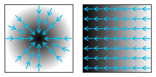
In vector calculus, the gradient of a scalar-valued differentiable function of several variables is the vector field whose value at a point is the "direction and rate of fastest increase". If the gradient of a function is non-zero at a point , the direction of the gradient is the direction in which the function increases most quickly from , and the magnitude of the gradient is the rate of increase in that direction, the greatest absolute directional derivative. Further, a point where the gradient is the zero vector is known as a stationary point. The gradient thus plays a fundamental role in optimization theory, where it is used to maximize a function by gradient ascent. In coordinate-free terms, the gradient of a function may be defined by:
In probability theory, the central limit theorem (CLT) establishes that, in many situations, for independent and identically distributed random variables, the sampling distribution of the standardized sample mean tends towards the standard normal distribution even if the original variables themselves are not normally distributed.
The likelihood function is the joint probability of observed data viewed as a function of the parameters of a statistical model.
In mathematics, a partial derivative of a function of several variables is its derivative with respect to one of those variables, with the others held constant. Partial derivatives are used in vector calculus and differential geometry.
In statistics, maximum likelihood estimation (MLE) is a method of estimating the parameters of an assumed probability distribution, given some observed data. This is achieved by maximizing a likelihood function so that, under the assumed statistical model, the observed data is most probable. The point in the parameter space that maximizes the likelihood function is called the maximum likelihood estimate. The logic of maximum likelihood is both intuitive and flexible, and as such the method has become a dominant means of statistical inference.
In vector calculus, the divergence theorem, also known as Gauss's theorem or Ostrogradsky's theorem, is a theorem which relates the flux of a vector field through a closed surface to the divergence of the field in the volume enclosed.
In vector calculus, the Jacobian matrix of a vector-valued function of several variables is the matrix of all its first-order partial derivatives. When this matrix is square, that is, when the function takes the same number of variables as input as the number of vector components of its output, its determinant is referred to as the Jacobian determinant. Both the matrix and the determinant are often referred to simply as the Jacobian in literature.
In vector calculus, Green's theorem relates a line integral around a simple closed curve C to a double integral over the plane region D bounded by C. It is the two-dimensional special case of Stokes' theorem.
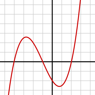
In mathematics, a differentiable function of one real variable is a function whose derivative exists at each point in its domain. In other words, the graph of a differentiable function has a non-vertical tangent line at each interior point in its domain. A differentiable function is smooth and does not contain any break, angle, or cusp.
In mathematics, the Hessian matrix, Hessian or Hesse matrix is a square matrix of second-order partial derivatives of a scalar-valued function, or scalar field. It describes the local curvature of a function of many variables. The Hessian matrix was developed in the 19th century by the German mathematician Ludwig Otto Hesse and later named after him. Hesse originally used the term "functional determinants". The Hessian is sometimes denoted by H or, ambiguously, by ∇2.
In mathematics, a homogeneous function is a function of several variables such that, if all its arguments are multiplied by a scalar, then its value is multiplied by some power of this scalar, called the degree of homogeneity, or simply the degree; that is, if k is an integer, a function f of n variables is homogeneous of degree k if
In mathematics, a norm is a function from a real or complex vector space to the non-negative real numbers that behaves in certain ways like the distance from the origin: it commutes with scaling, obeys a form of the triangle inequality, and is zero only at the origin. In particular, the Euclidean distance in a Euclidean space is defined by a norm on the associated Euclidean vector space, called the Euclidean norm, the 2-norm, or, sometimes, the magnitude of the vector. This norm can be defined as the square root of the inner product of a vector with itself.
In mathematics, the Helmholtz equation is the eigenvalue problem for the Laplace operator. It corresponds to the linear partial differential equation

The Ramsey–Cass–Koopmans model, or Ramsey growth model, is a neoclassical model of economic growth based primarily on the work of Frank P. Ramsey, with significant extensions by David Cass and Tjalling Koopmans. The Ramsey–Cass–Koopmans model differs from the Solow–Swan model in that the choice of consumption is explicitly microfounded at a point in time and so endogenizes the savings rate. As a result, unlike in the Solow–Swan model, the saving rate may not be constant along the transition to the long run steady state. Another implication of the model is that the outcome is Pareto optimal or Pareto efficient.

The Navier–Stokes existence and smoothness problem concerns the mathematical properties of solutions to the Navier–Stokes equations, a system of partial differential equations that describe the motion of a fluid in space. Solutions to the Navier–Stokes equations are used in many practical applications. However, theoretical understanding of the solutions to these equations is incomplete. In particular, solutions of the Navier–Stokes equations often include turbulence, which remains one of the greatest unsolved problems in physics, despite its immense importance in science and engineering.
In applied mathematics, polyharmonic splines are used for function approximation and data interpolation. They are very useful for interpolating and fitting scattered data in many dimensions. Special cases include thin plate splines and natural cubic splines in one dimension.
Stochastic portfolio theory (SPT) is a mathematical theory for analyzing stock market structure and portfolio behavior introduced by E. Robert Fernholz in 2002. It is descriptive as opposed to normative, and is consistent with the observed behavior of actual markets. Normative assumptions, which serve as a basis for earlier theories like modern portfolio theory (MPT) and the capital asset pricing model (CAPM), are absent from SPT.
In the science of fluid flow, Stokes' paradox is the phenomenon that there can be no creeping flow of a fluid around a disk in two dimensions; or, equivalently, the fact there is no non-trivial steady-state solution for the Stokes equations around an infinitely long cylinder. This is opposed to the 3-dimensional case, where Stokes' method provides a solution to the problem of flow around a sphere.
Uzawa's theorem, also known as the steady state growth theorem, is a theorem in economic growth theory concerning the form that technological change can take in the Solow–Swan and Ramsey–Cass–Koopmans growth models. It was first proved by Japanese economist Hirofumi Uzawa.


