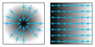
In vector calculus, the gradient of a scalar-valued differentiable function of several variables is the vector field whose value at a point gives the direction and the rate of fastest increase. The gradient transforms like a vector under change of basis of the space of variables of . If the gradient of a function is non-zero at a point , the direction of the gradient is the direction in which the function increases most quickly from , and the magnitude of the gradient is the rate of increase in that direction, the greatest absolute directional derivative. Further, a point where the gradient is the zero vector is known as a stationary point. The gradient thus plays a fundamental role in optimization theory, where it is used to minimize a function by gradient descent. In coordinate-free terms, the gradient of a function may be defined by:

In the mathematical field of numerical analysis, interpolation is a type of estimation, a method of constructing (finding) new data points based on the range of a discrete set of known data points.

In the mathematical subfield of numerical analysis, a B-spline or basis spline is a spline function that has minimal support with respect to a given degree, smoothness, and domain partition. Any spline function of given degree can be expressed as a linear combination of B-splines of that degree. Cardinal B-splines have knots that are equidistant from each other. B-splines can be used for curve-fitting and numerical differentiation of experimental data.
In mathematics, an operator is generally a mapping or function that acts on elements of a space to produce elements of another space. There is no general definition of an operator, but the term is often used in place of function when the domain is a set of functions or other structured objects. Also, the domain of an operator is often difficult to characterize explicitly, and may be extended so as to act on related objects. See Operator (physics) for other examples.
In mathematics, a tangent vector is a vector that is tangent to a curve or surface at a given point. Tangent vectors are described in the differential geometry of curves in the context of curves in Rn. More generally, tangent vectors are elements of a tangent space of a differentiable manifold. Tangent vectors can also be described in terms of germs. Formally, a tangent vector at the point is a linear derivation of the algebra defined by the set of germs at .
In numerical analysis, polynomial interpolation is the interpolation of a given bivariate data set by the polynomial of lowest possible degree that passes through the points of the dataset.

In statistics, originally in geostatistics, kriging or Kriging, also known as Gaussian process regression, is a method of interpolation based on Gaussian process governed by prior covariances. Under suitable assumptions of the prior, kriging gives the best linear unbiased prediction (BLUP) at unsampled locations. Interpolating methods based on other criteria such as smoothness may not yield the BLUP. The method is widely used in the domain of spatial analysis and computer experiments. The technique is also known as Wiener–Kolmogorov prediction, after Norbert Wiener and Andrey Kolmogorov.
In mathematics, the Riesz–Thorin theorem, often referred to as the Riesz–Thorin interpolation theorem or the Riesz–Thorin convexity theorem, is a result about interpolation of operators. It is named after Marcel Riesz and his student G. Olof Thorin.
In statistics, the theory of minimum norm quadratic unbiased estimation (MINQUE) was developed by C. R. Rao. MINQUE is a theory alongside other estimation methods in estimation theory, such as the method of moments or maximum likelihood estimation. Similar to the theory of best linear unbiased estimation, MINQUE is specifically concerned with linear regression models. The method was originally conceived to estimate heteroscedastic error variance in multiple linear regression. MINQUE estimators also provide an alternative to maximum likelihood estimators or restricted maximum likelihood estimators for variance components in mixed effects models. MINQUE estimators are quadratic forms of the response variable and are used to estimate a linear function of the variances.
Inversive congruential generators are a type of nonlinear congruential pseudorandom number generator, which use the modular multiplicative inverse to generate the next number in a sequence. The standard formula for an inversive congruential generator, modulo some prime q is:
In mathematics a radial basis function (RBF) is a real-valued function whose value depends only on the distance between the input and some fixed point, either the origin, so that , or some other fixed point , called a center, so that . Any function that satisfies the property is a radial function. The distance is usually Euclidean distance, although other metrics are sometimes used. They are often used as a collection which forms a basis for some function space of interest, hence the name.

In geometry, a three-dimensional space is a mathematical space in which three values (coordinates) are required to determine the position of a point. Most commonly, it is the three-dimensional Euclidean space, that is, the Euclidean space of dimension three, which models physical space. More general three-dimensional spaces are called 3-manifolds. The term may also refer colloquially to a subset of space, a three-dimensional region, a solid figure.

The Navier–Stokes existence and smoothness problem concerns the mathematical properties of solutions to the Navier–Stokes equations, a system of partial differential equations that describe the motion of a fluid in space. Solutions to the Navier–Stokes equations are used in many practical applications. However, theoretical understanding of the solutions to these equations is incomplete. In particular, solutions of the Navier–Stokes equations often include turbulence, which remains one of the greatest unsolved problems in physics, despite its immense importance in science and engineering.
In applied mathematics, polyharmonic splines are used for function approximation and data interpolation. They are very useful for interpolating and fitting scattered data in many dimensions. Special cases include thin plate splines and natural cubic splines in one dimension.

Natural neighbor interpolation is a method of spatial interpolation, developed by Robin Sibson. The method is based on Voronoi tessellation of a discrete set of spatial points. This has advantages over simpler methods of interpolation, such as nearest-neighbor interpolation, in that it provides a smoother approximation to the underlying "true" function.
In numerical analysis, multivariate interpolation is interpolation on functions of more than one variable ; when the variates are spatial coordinates, it is also known as spatial interpolation.
In the field of mathematical modeling, a radial basis function network is an artificial neural network that uses radial basis functions as activation functions. The output of the network is a linear combination of radial basis functions of the inputs and neuron parameters. Radial basis function networks have many uses, including function approximation, time series prediction, classification, and system control. They were first formulated in a 1988 paper by Broomhead and Lowe, both researchers at the Royal Signals and Radar Establishment.
In operator theory, a branch of mathematics, a positive-definite kernel is a generalization of a positive-definite function or a positive-definite matrix. It was first introduced by James Mercer in the early 20th century, in the context of solving integral operator equations. Since then, positive-definite functions and their various analogues and generalizations have arisen in diverse parts of mathematics. They occur naturally in Fourier analysis, probability theory, operator theory, complex function-theory, moment problems, integral equations, boundary-value problems for partial differential equations, machine learning, embedding problem, information theory, and other areas.
Barnes interpolation, named after Stanley L. Barnes, is the interpolation of unevenly spread data points from a set of measurements of an unknown function in two dimensions into an analytic function of two variables. An example of a situation where the Barnes scheme is important is in weather forecasting where measurements are made wherever monitoring stations may be located, the positions of which are constrained by topography. Such interpolation is essential in data visualisation, e.g. in the construction of contour plots or other representations of analytic surfaces.
Steered-response power (SRP) is a family of acoustic source localization algorithms that can be interpreted as a beamforming-based approach that searches for the candidate position or direction that maximizes the output of a steered delay-and-sum beamformer.


![Shepard's interpolation for different power parameters p, from scattered points on the surface
z
=
exp
[?]
(
-
x
2
-
y
2
)
{\displaystyle z=\exp(-x^{2}-y^{2})} Shepard interpolation 2.png](http://upload.wikimedia.org/wikipedia/commons/7/71/Shepard_interpolation_2.png)


