Isoquant

Last updated
An isoquant map where production output Q3 > Q2 > Q1. Typically inputs X and Y would refer to labor and capital respectively. More of input X, input Y, or both is required to move from isoquant Q1 to Q2, or from Q2 to Q3. Isoquant map.png
An isoquant map where production output Q3 > Q2 > Q1. Typically inputs X and Y would refer to labor and capital respectively. More of input X, input Y, or both is required to move from isoquant Q1 to Q2, or from Q2 to Q3.
A) Example of an isoquant map with two inputs that are perfect substitutes. Isoquant perfectsubs.png
A) Example of an isoquant map with two inputs that are perfect substitutes.
B) Example of an isoquant map with two inputs that are perfect complements. Isoquant perfect compliments.png
B) Example of an isoquant map with two inputs that are perfect complements.

An isoquant (derived from quantity and the Greek word iso, meaning equal), in microeconomics, is a contour line drawn through the set of points at which the same quantity of output is produced while changing the quantities of two or more inputs. [1] [2] The x and y axis on an isoquant represent two relevant inputs, which are usually a factor of production such as labour, capital, land, or organisation. An isoquant may also be known as an “Iso-Product Curve”, or an “Equal Product Curve”.

Contents

Isoquants vs. indifference curves

While an indifference curve mapping helps to solve the utility-maximizing problem of consumers, the isoquant mapping deals with the cost-minimization and profit and output maximisation problem of producers. Indifference curves further differ to isoquants, in that they cannot offer a precise measurement of utility, only how it is relevant to a baseline. Whereas, from an isoquant, the product can be measured accurately in physical units, and it is known by exactly how much isoquant 1 exceeds isoquant 2.

Nature and practical uses

In managerial economics, isoquants are typically drawn along with isocost curves in capital-labor graphs, showing the technological tradeoff between capital and labor in the production function, and the decreasing marginal returns of both inputs. In managerial economics, the unit of isoquant is commonly the net of capital cost. As such, isoquants by nature are downward sloping due to operation of diminishing marginal rates of technical substitution (MRTS). [3] [4] The slope of an isoquant represents the rate at which input x can be substituted for input y. [5] This concept is the MRTS, so MRTS=slope of the isoquant. Thus, the steeper the isoquant, the higher the MRTS. Since MRTS must diminish, isoquants must be convex to their origin. Adding one input while holding the other constant eventually leads to decreasing marginal output.

The contour line of an isoquant represents every combination of two inputs which fully maximise a firms’ use of resources (such as budget, or time). Full maximisation of resources is usually considered ‘efficient’. Efficient allocation of factors of production occur only when two isoquants are tangent to one another. If a firm produces to the left of the contour line, then the firm is considered to be operating inefficiently, because they are not maximising use of their available resources. [6] A firm cannot produce to the right of the contour line unless they exceed their constraints.

D) Production isoquant (strictly convex) and isocost curve (linear) TE-Production-Isoquant.png
D) Production isoquant (strictly convex) and isocost curve (linear)

A family of isoquants can be represented by an isoquant map, a graph combining a number of isoquants, each representing a different quantity of output.An isoquant map can indicate decreasing or increasing returns to scale based on increasing or decreasing distances between the isoquant pairs of fixed output increment, as output increases. [7] If the distance between those isoquants increases as output increases, the firm's production function is exhibiting decreasing returns to scale; doubling both inputs will result in placement on an isoquant with less than double the output of the previous isoquant. Conversely, if the distance is decreasing as output increases, the firm is experiencing increasing returns to scale; doubling both inputs results in placement on an isoquant with more than twice the output of the original isoquant. A firm can choose to utilise the information an isoquant gives on returns to scale, by using it as insight how to allocate resources. [8]

C) Isoquant 1 is much more input-Y intensive than isoquant 2. Isoquant x vs y input intensity.jpg
C) Isoquant 1 is much more input-Y intensive than isoquant 2.

Knowing how to allocate resources is a concept pertinent to managerial economics. Isoquants can be useful to graphically represent this issue of scarcity. They show the extent to which the firm in question has the ability to substitute between two different inputs (x and y in the graph) at will in order to produce the same level of output (see: Graph C)). They also represent different quantity combinations of two goods which adhere to a budget constraint. Thus, they can be used as a tool to help management make better informed decisions regarding production and profit dilemmas, such as cost or waste minimization, and revenue and output maximization.

A firm can determine the least cost combination of inputs to produce a given output, by combining isocost curves and isoquants, and adhering to First Order Conditions. [3] The least cost combination is where the ratio of marginal products is equal to the ratio of factor prices. At this point, the slope of the isoquant, and the slope of the isocost, will be equal (see intersection of graph D). A firm has incentive to produce at the least cost combination because it is at this point, the related costs of desired production are minimised. [9]

As with indifference curves, two isoquants can never cross. Also, every possible combination of inputs is on an isoquant. Finally, any combination of inputs above or to the right of an isoquant results represents a higher level of output, and vice versa. Although the marginal product of an input decreases as you increase the quantity of the input while holding all other inputs constant, the marginal product is never negative in the empirically observed range since a rational firm would never increase an input to decrease output.

Shapes

If the two inputs are perfect substitutes, the resulting isoquant map generated is represented in fig. A; with a given level of production Q3, input X can be replaced by input Y at an unchanging rate. The perfect substitute inputs do not experience decreasing marginal rates of return when they are substituted for each other in the production function.

If the two inputs are perfect complements, the isoquant map takes the form of fig. B; with a level of production Q3, input X and input Y can only be combined efficiently in the certain ratio occurring at the kink in the isoquant. The firm will combine the two inputs in the required ratio to maximize profit.

Isoquants are typically combined with isocost lines in order to solve a cost-minimization problem for given level of output. In the typical case shown in the top figure, with smoothly curved isoquants, a firm with fixed unit costs of the inputs will have isocost curves that are linear and downward sloped; any point of tangency between an isoquant and an isocost curve represents the cost-minimizing input combination for producing the output level associated with that isoquant. A line joining tangency points of isoquants and isocosts (with input prices held constant) is called the expansion path. [10]

Non-convexity

Under the assumption of declining marginal rate of technical substitution, and hence a positive and finite elasticity of substitution, the isoquant is convex to the origin. A locally nonconvex isoquant can occur if there are sufficiently strong returns to scale in one of the inputs. In this case, there is a negative elasticity of substitution - as the ratio of input A to input B increases, the marginal product of A relative to B increases rather than decreases.

A nonconvex isoquant is prone to produce large and discontinuous changes in the price minimizing input mix in response to price changes. Consider for example the case where the isoquant is globally nonconvex, and the isocost curve is linear. In this case the minimum cost mix of inputs will be a corner solution, and include only one input (for example either input A or input B). The choice of which input to use will depend on the relative prices. At some critical price ratio, the optimum input mix will shift from all input A to all input B and vice versa in response to a small change in relative prices.

See also

Related Research Articles

Physical capital represents in economics one of the three primary factors of production. Physical capital is the apparatus used to produce a good and services. Physical capital represents the tangible man-made goods that help and support the production. Inventory, cash, equipment or real estate are all examples of physical capital.

<span class="mw-page-title-main">Profit maximization</span> Process to determine the highest profits for a firm

In economics, profit maximization is the short run or long run process by which a firm may determine the price, input and output levels that will lead to the highest possible total profit. In neoclassical economics, which is currently the mainstream approach to microeconomics, the firm is assumed to be a "rational agent" which wants to maximize its total profit, which is the difference between its total revenue and its total cost.

The following outline is provided as an overview of and topical guide to industrial organization:

In economics, the marginal cost is the change in the total cost that arises when the quantity produced is incremented, the cost of producing additional quantity. In some contexts, it refers to an increment of one unit of output, and in others it refers to the rate of change of total cost as output is increased by an infinitesimal amount. As Figure 1 shows, the marginal cost is measured in dollars per unit, whereas total cost is in dollars, and the marginal cost is the slope of the total cost, the rate at which it increases with output. Marginal cost is different from average cost, which is the total cost divided by the number of units produced.

<span class="mw-page-title-main">Production–possibility frontier</span> Visualization of all possible options of output for a two-good economy

In microeconomics, a production–possibility frontier (PPF), production possibility curve (PPC), or production possibility boundary (PPB) is a graphical representation showing all the possible options of output for two goods that can be produced using all factors of production, where the given resources are fully and efficiently utilized per unit time. A PPF illustrates several economic concepts, such as allocative efficiency, economies of scale, opportunity cost, productive efficiency, and scarcity of resources.

<span class="mw-page-title-main">Production function</span> Used to define marginal product and to distinguish allocative efficiency

In economics, a production function gives the technological relation between quantities of physical inputs and quantities of output of goods. The production function is one of the key concepts of mainstream neoclassical theories, used to define marginal product and to distinguish allocative efficiency, a key focus of economics. One important purpose of the production function is to address allocative efficiency in the use of factor inputs in production and the resulting distribution of income to those factors, while abstracting away from the technological problems of achieving technical efficiency, as an engineer or professional manager might understand it.

In economics, average cost or unit cost is equal to total cost (TC) divided by the number of units of a good produced :

<span class="mw-page-title-main">Demand curve</span> Graph of how much of something a consumer would buy at a certain price

In a demand schedule, a demand curve is a graph depicting the relationship between the price of a certain commodity and the quantity of that commodity that is demanded at that price. Demand curves can be used either for the price-quantity relationship for an individual consumer, or for all consumers in a particular market.

<span class="mw-page-title-main">Marginal revenue</span> Additional total revenue generated by increasing product sales by 1 unit

Marginal revenue is a central concept in microeconomics that describes the additional total revenue generated by increasing product sales by 1 unit. Marginal revenue is the increase in revenue from the sale of one additional unit of product, i.e., the revenue from the sale of the last unit of product. It can be positive or negative. Marginal revenue is an important concept in vendor analysis. To derive the value of marginal revenue, it is required to examine the difference between the aggregate benefits a firm received from the quantity of a good and service produced last period and the current period with one extra unit increase in the rate of production. Marginal revenue is a fundamental tool for economic decision making within a firm's setting, together with marginal cost to be considered.

<span class="mw-page-title-main">Isocost</span>

In economics, an isocost line shows all combinations of inputs which cost the same total amount. Although similar to the budget constraint in consumer theory, the use of the isocost line pertains to cost-minimization in production, as opposed to utility-maximization. For the two production inputs labour and capital, with fixed unit costs of the inputs, the equation of the isocost line is

In economics, a cost curve is a graph of the costs of production as a function of total quantity produced. In a free market economy, productively efficient firms optimize their production process by minimizing cost consistent with each possible level of production, and the result is a cost curve. Profit-maximizing firms use cost curves to decide output quantities. There are various types of cost curves, all related to each other, including total and average cost curves; marginal cost curves, which are equal to the differential of the total cost curves; and variable cost curves. Some are applicable to the short run, others to the long run.

In economics, a conditional factor demand is the cost-minimizing level of an input such as labor or capital, required to produce a given level of output, for given unit input costs of the input factors. A conditional factor demand function expresses the conditional factor demand as a function of the output level and the input costs. The conditional portion of this phrase refers to the fact that this function is conditional on a given level of output, so output is one argument of the function. Typically this concept arises in a long run context in which both labor and capital usage are choosable by the firm, so a single optimization gives rise to conditional factor demands for each of labor and capital.

<span class="mw-page-title-main">Marginal rate of technical substitution</span>

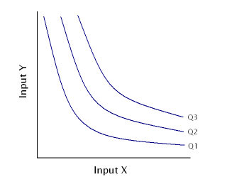
In microeconomic theory, the marginal rate of technical substitution (MRTS)—or technical rate of substitution (TRS)—is the amount by which the quantity of one input has to be reduced when one extra unit of another input is used, so that output remains constant.

<span class="mw-page-title-main">Supply (economics)</span> Amount of a good that sellers are willing to provide in the market

In economics, supply is the amount of a resource that firms, producers, labourers, providers of financial assets, or other economic agents are willing and able to provide to the marketplace or to an individual. Supply can be in produced goods, labour time, raw materials, or any other scarce or valuable object. Supply is often plotted graphically as a supply curve, with the price per unit on the vertical axis and quantity supplied as a function of price on the horizontal axis. This reversal of the usual position of the dependent variable and the independent variable is an unfortunate but standard convention.

Within economics, margin is a concept used to describe the current level of consumption or production of a good or service. Margin also encompasses various concepts within economics, denoted as marginal concepts, which are used to explain the specific change in the quantity of goods and services produced and consumed. These concepts are central to the economic theory of marginalism. This is a theory that states that economic decisions are made in reference to incremental units at the margin, and it further suggests that the decision on whether an individual or entity will obtain additional units of a good or service depending on the marginal utility of the product.

In economics, the marginal product of capital (MPK) is the additional production that a firm experiences when it adds an extra unit of capital. It is a feature of the production function, alongside the labour input.

<span class="mw-page-title-main">Factor market</span> In economics, a market where resources used in the production process are bought and sold

In economics, a factor market is a market where factors of production are bought and sold. Factor markets allocate factors of production, including land, labour and capital, and distribute income to the owners of productive resources, such as wages, rents, etc.

In economics, the marginal product of labor (MPL) is the change in output that results from employing an added unit of labor. It is a feature of the production function, and depends on the amounts of physical capital and labor already in use.

A Robinson Crusoe economy is a simple framework used to study some fundamental issues in economics. It assumes an economy with one consumer, one producer and two goods. The title "Robinson Crusoe" is a reference to the 1719 novel of the same name authored by Daniel Defoe.

<span class="mw-page-title-main">Expansion path</span>

In economics, an expansion path is a path connecting optimal input combinations as the scale of production expands. which is often represented as a curve in a graph with quantities of two inputs, typically physical capital and labor, plotted on the axes. A producer seeking to produce a given number of units of a product in the cheapest possible way chooses the point on the expansion path that is also on the isoquant associated with that output level.

References

  1. Varian, Hal R. (1992). Microeconomic Analysis (Third ed.). Norton. ISBN   0-393-95735-7.
  2. Chiang, Alpha C. (1984). Fundamental Methods of Mathematical Economics (Third ed.). McGraw-Hill. pp. 359–363. ISBN   0-07-010813-7.
  3. 1 2 www2.econ.iastate.edu http://www2.econ.iastate.edu/classes/econ101/choi/ch11d.htm . Retrieved 2021-04-25.{{cite web}}: Missing or empty |title= (help)
  4. "Isoquants". www.economics.utoronto.ca. Retrieved 2021-04-25.
  5. "Production Functions" (PDF). UCLA. n.d. Retrieved 25 April 2021.{{cite web}}: CS1 maint: url-status (link)
  6. Arrow, K. J.; Chenery, H. B.; Minhas, B. S.; Solow, R. M. (1961). "Capital-Labor Substitution and Economic Efficiency". The Review of Economics and Statistics. 43 (3): 225–250. doi:10.2307/1927286. ISSN   0034-6535. JSTOR   1927286.
  7. Kwatiah, Natasha (2016-03-02). "The Laws of Returns to Scale in Terms of Isoquant Approach". Economics Discussion. Retrieved 2021-04-25.
  8. "The Discovery of the Isoquant". ResearchGate. Retrieved 2021-04-25.
  9. "Expansion path, ridgeline and least cost combination of inputs" (PDF). Eagri. n.d. Retrieved 2021-04-25.{{cite web}}: CS1 maint: url-status (link)
  10. Salvatore, Dominick (1989). Schaum's outline of theory and problems of managerial economics, McGraw-Hill, ISBN   978-0-07-054513-7